← 2023 Answer | 🏠 Index | 2018–2024 Repeated Questions →

---

ECE 2207: 2024 Semester Final: Explanation Style Answers

RUET · ECE Dept · 2nd Year Even Semester (Session 2023-24)

Deep tutorial-style explanations focusing on first-principles physics, "why over what", step-by-step logic, and practical engineering intuition. Core cross-cutting theory topics are detailed in 2018_2024_answer.md.

---

Question 1

Q1(a): Transformer Schematic and Physical Meaning of Variables

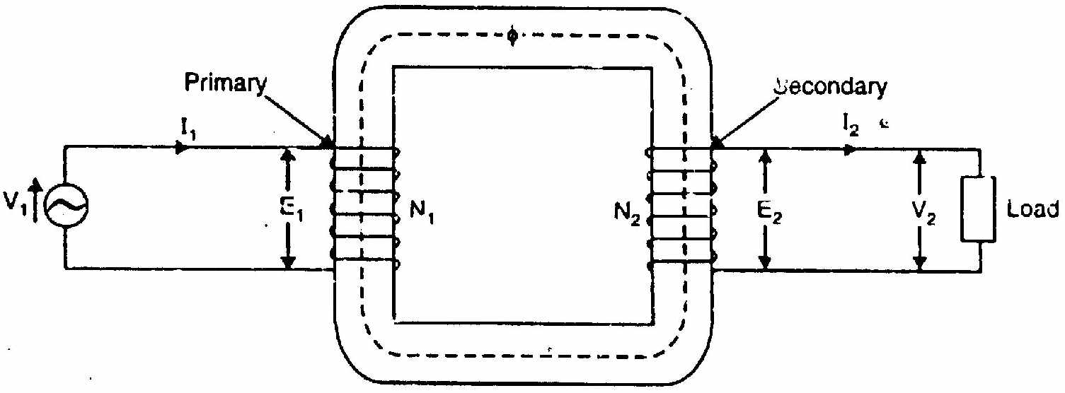
What each variable represents physically

A transformer is fundamentally two electric circuits coupled through a common magnetic circuit. Understanding the physical role of each variable avoids mixing up applied vs induced quantities:

1. Primary Applied Voltage $v_1(t),V_1$: The external driving potential supplied by the generator or grid. It forces an alternating current to flow through the primary coil.
2. Primary Counter-EMF $e_1(t),E_1$: The self-induced voltage produced in the primary coil by the alternating core flux $\Phi (t)$. By Faraday's and Lenz's laws, $e_1(t)=-N_1\frac{d\Phi }{dt}$. In an ideal transformer, this self-induced EMF exactly opposes and balances the applied voltage ($V_1=-E_1$). It acts as the "governor" of the transformer: when secondary load increases, the flux tries to dip, $E_1$ decreases slightly, allowing more primary current $I_1$ to rush in from the source.
3. Mutual Core Flux $\Phi (t)={\Phi }_m\sin \omega t$: The common magnetic flux confined almost entirely within the high-permeability laminated steel core. This flux links all $N_1$ turns of the primary and all $N_2$ turns of the secondary, serving as the energy transfer bridge between the two electrically isolated circuits.
4. Secondary Induced EMF $e_2(t),E_2$: The mutually induced EMF in the secondary coil: $e_2(t)=-N_2\frac{d\Phi }{dt}$. Because both windings share the exact same mutual flux, the EMF induced per turn is identical: $E_1/N_1=E_2/N_2=4.44f{\Phi }_m$.
5. Secondary Terminal Voltage $v_2(t),V_2$: The actual voltage available across the secondary load terminals. In an ideal transformer, $V_2=E_2$. In a practical transformer, $V_2=E_2-I_2(R_2+j{X}_2)$ due to internal impedance drops.
6. Secondary Load Current $i_2(t),I_2$: The current drawn by load impedance $Z_L$. Its magnitude and phase angle ${\theta }_2$ depend entirely on the load nature ($Z_L=R_L+j{X}_L$).
7. Primary Load Component Current $I_2^{\prime }$: As soon as $I_2$ flows, it creates a demagnetizing MMF ($N_2{I}_2$) in the core. To maintain constant core flux ${\Phi }_m$, the primary immediately draws an equal and opposite balancing current $I_2^{\prime }$ such that $N_1{I}_2^{\prime }=N_2{I}_2⟹I_2^{\prime }=K{I}_2$.
8. Transformation Ratio $K=N_2/N_1=E_2/E_1$: Governs voltage stepping. If $K>1$, it is a step-up transformer; if $K<1$, step-down. Current transforms inversely ($I_1^{\prime }/I_2=K$).

---

Q1(b): No-Load Operation of a 1-Phase Transformer

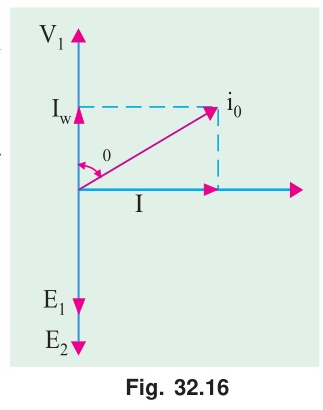
What happens physically before the load is connected

When you switch on the transformer with the secondary open ($I_2=0$), the primary winding is simply an iron-cored inductor connected to an AC voltage source.

The primary draws a very small current called the no-load current $I_0$ (typically 2% to 10% of rated full-load current). Why doesn't an enormous short-circuit current flow, even though the copper resistance $R_1$ is tiny? Because the alternating flux creates a massive counter-EMF $E_1\approx V_1$ that throttles the current.

The small current $I_0$ performs two distinct physical tasks:

1. Magnetizing Role ($I_m$): Creates and sustains the alternating magnetic field in the core. Because the iron core requires energy to build up flux and releases it when flux collapses, this is pure reactive energy. $I_m$ lags the applied voltage $V_1$ by 90° (it is in phase with the flux ${\Phi }_m$).
2. Loss-Supplying Role ($I_c$): As the core flux cycles back and forth at 50 Hz, magnetic domains continually reorient (hysteresis loss) and small circulating eddy currents swirl in the steel sheets (eddy current loss). These generate heat in the core. The active current $I_c$ is in phase with $V_1$ and draws real power from the source to supply these core losses ($P_c=V_1{I}_c$).

The total no-load current is the phasor sum: $$I_0=I_c+I_m,I_0=\sqrt{I_c^2+I_m^2}$$ Because $I_m\gg I_c$ in iron-core transformers, $I_0$ lags $V_1$ by a large angle ${\varphi }_0\approx 70°\text{–}85°$ (very poor no-load power factor $\cos {\varphi }_0\approx 0.1\text{–}0.3$).

Step-by-step construction of the no-load phasor diagram

1. Reference Phasor: Draw core flux ${\Phi }_m$ along the positive horizontal axis. Flux is the fundamental state variable that couples primary and secondary.
2. Induced EMFs: By Faraday's law ($e=-N\frac{d\Phi }{dt}=\omega N{\Phi }_m\sin (\omega t-90°)$), both self-induced EMF $E_1$ and mutually induced EMF $E_2$ lag the flux ${\Phi }_m$ by 90°. Draw $E_1$ and $E_2$ vertically downward.
3. Primary Counter-Voltage: For an ideal winding with zero resistance, applied voltage must exactly oppose the counter-EMF: $V_1=-E_1$. Draw $V_1$ vertically upward (leading flux by 90°).
4. Current Components:
   • Draw $I_c$ along $+V_1$ (active component in phase with voltage).
   • Draw $I_m$ along $+{\Phi }_m$ (quadrature component in phase with flux, 90° behind $V_1$).
5. No-load Current: Complete the rectangle to find $I_0=I_c+I_m$.
6. Secondary Terminal Voltage: With secondary open, no drop occurs across secondary winding resistance or leakage reactance, so $V_2=E_2$ (downward, 180° out of phase with $V_1$).

---

Question 2

Q2(a): Phasor Diagram of R-L Loaded Ideal Transformer

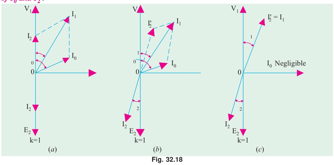
Physical story of how a transformer reacts to an inductive load

In an ideal transformer, we assume:

• Zero winding resistance ($R_1=R_2=0$) $⟹$ no $I^{2}R$ copper losses.
• Zero leakage flux ($X_1=X_2=0$) $⟹$ all flux stays strictly within the core.
• Infinite core permeability and zero core loss $⟹I_0\approx 0$ (magnetizing current is negligible compared to load current).

When an R-L (inductive) load is connected to the secondary terminals:

1. Secondary terminal voltage and current: The secondary induced EMF $E_2$ appears directly across the load ($V_2=E_2$). Because the load has inductive reactance ($Z_L=R_L+j{X}_L$), the secondary current $I_2$ lags secondary voltage $V_2$ by the load impedance angle: $${\theta }_2={\tan }^{-1}\left(\frac{X_L}{R_L}\right)$$
2. The MMF balance struggle: Secondary current $I_2$ flowing through $N_2$ turns sets up a demagnetizing secondary MMF $F_2=N_2{I}_2$. If unopposed, this MMF would immediately reduce the mutual core flux ${\Phi }_m$.
3. Primary response: Any drop in core flux instantly lowers the counter-EMF $E_1$. The applied supply voltage $V_1$ now exceeds $E_1$, forcing an additional balancing current $I_1$ into the primary winding. The primary develops a balancing MMF $F_1=N_1{I}_1$ such that: $$N_1{I}_1+N_2{I}_2=0⟹I_1=-\frac{N_2}{N_1}{I}_2=-K{I}_2$$ Thus, the primary current is in exact anti-phase (180° reversed) to the secondary current.

Step-by-step phasor construction

Step	Phasor	Direction / Position	Physical Justification
1	${\Phi }_m$	Horizontal (+X axis, 0°)	Common mutual flux chosen as the reference.
2	$E_1,E_2$	Vertically downward (−90°)	Faraday's law derivative introduces a −90° phase shift relative to flux.
3	$V_2$	Coincident with $E_2$ (−90°)	In an ideal secondary winding, internal impedance drop is zero.
4	$I_2$	Clockwise from $V_2$ by ${\theta }_2$ (−90° − ${\theta }_2$)	Inductive load draws current that lags load voltage by ${\theta }_2={\tan }^{-1}(X_L/R_L)$.
5	$V_1$	Vertically upward (+90°)	Applied voltage must exactly balance counter-EMF ($V_1=-E_1$).
6	$I_1$	Quadrant II (+90° − ${\theta }_2$)	Primary current is in exact anti-phase with $I_2$ to balance secondary MMF.

Key Insight: The angle between $V_1$ (+90°) and $I_1$ (+90° − ${\theta }_2$) is exactly ${\theta }_1={\theta }_2$. The ideal transformer reflects the load power factor angle perfectly to the source: $\cos {\theta }_1=\cos {\theta }_2$.

---

Q2(b): Leakage Flux and Its Effect on Transformer Operation

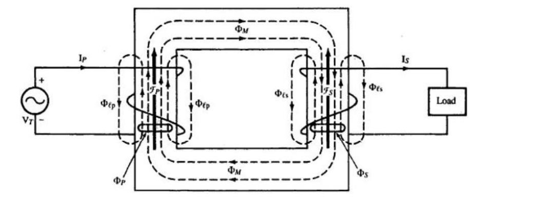
For full physical derivation and diagrams see T-02: Leakage Flux: Physical Picture and All Effects.

Why leakage flux exists and how it behaves

In an actual transformer, not all magnetic lines of force stay entirely inside the core:

• Mutual Flux (${\Phi }_m$): Links both primary and secondary turns through the high-permeability iron path. This is the only flux that transfers energy between circuits.
• Primary Leakage Flux (${\Phi }_{l1}$): Links only primary turns $N_1$ and completes its loop through the surrounding air, insulation, and tank.
• Secondary Leakage Flux (${\Phi }_{l2}$): Links only secondary turns $N_2$ and completes its loop through air.

Four major effects on transformer operation:

1. Origin of Leakage Reactance ($X_1,X_2$): Because air has a constant magnetic permeability (${\mu }_0$), leakage flux does not saturate. It is strictly proportional to winding current (${\Phi }_{l1}\propto I_1$). By Faraday's law, this alternating leakage flux induces a self-inductance EMF $e_{l1}=-L_{l1}\frac{d{i}_1}{dt}$ which lags the current by 90°. In circuit analysis, this is modeled as an inductive leakage reactance: $$X_1=2\pi f{L}_{l1},X_2=2\pi f{L}_{l2}$$
2. Voltage Drops and Regulation: Leakage reactance drops voltage under load ($I_1{X}_1$ on primary, $I_2{X}_2$ on secondary). Under lagging power factor loads, the reactive drop $I_2{X}_2$ directly reduces secondary terminal voltage $V_2$, causing poor voltage regulation.
3. Reduction of Maximum Power Transfer: Leakage reactances form series impedances that limit the peak power and short-term overload capacity of the transformer.
4. Beneficial Role — Fault Current Limitation: If a dead short-circuit occurs on the secondary terminals, the only impedances limiting the catastrophic fault current are winding resistances and leakage reactances: $$I_{sc}=\frac{V_1}{\sqrt{R_{01}^2+X_{01}^2}}\approx \frac{V_1}{X_{01}}$$ Without leakage reactance, short-circuit current would reach destructive levels (hundreds of times rated current), tearing the windings apart via magnetic forces ($F\propto I^2$). Leakage reactance naturally throttles short-circuit current to a manageable 10–20 times rated current.

---

Question 3

Q3(a): Why OC and SC Tests Are Preferred Over Direct Loading

The physical and practical dilemma of direct loading

Testing a 100 kVA or 1000 kVA transformer by connecting an actual variable resistive/inductive load bank has severe drawbacks:

1. Immense Waste of Power: In a direct load test, full rated kVA must be supplied from the grid and converted entirely into waste heat in the load bank. For a 500 kVA unit, running a 4-hour temperature rise test wastes 2,000 kWh of energy.
2. Impracticality of Huge Variable Loads: Finding and wiring adjustable 3-phase load banks capable of drawing thousands of amperes at various power factors (0.8 lag, unity, 0.8 lead) is prohibitively expensive or physically impossible in a standard laboratory or factory floor.
3. Single Operating Point: Direct loading only measures performance at the specific load applied. To find efficiency at 25%, 50%, 75%, 100%, and 125% load, you must repeat the entire physical loading process multiple times.

The elegance of OC and SC tests: Virtual loading through loss separation

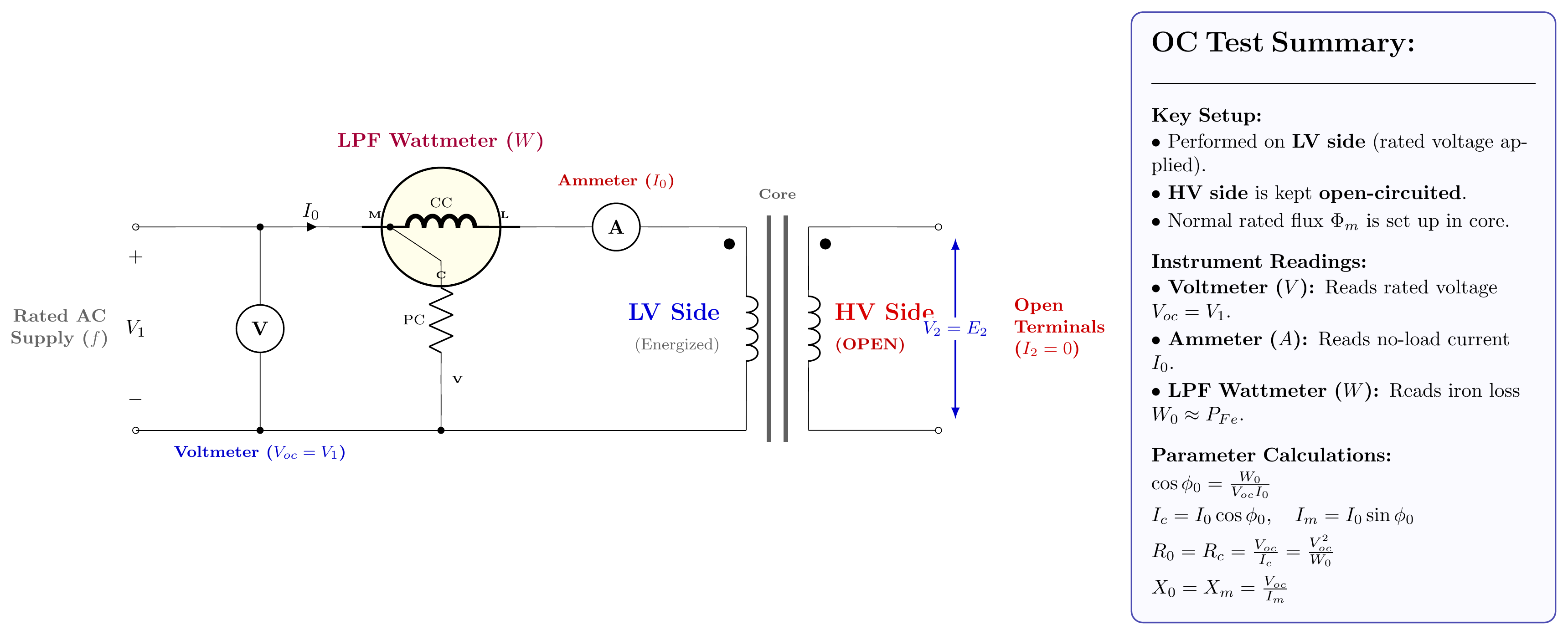
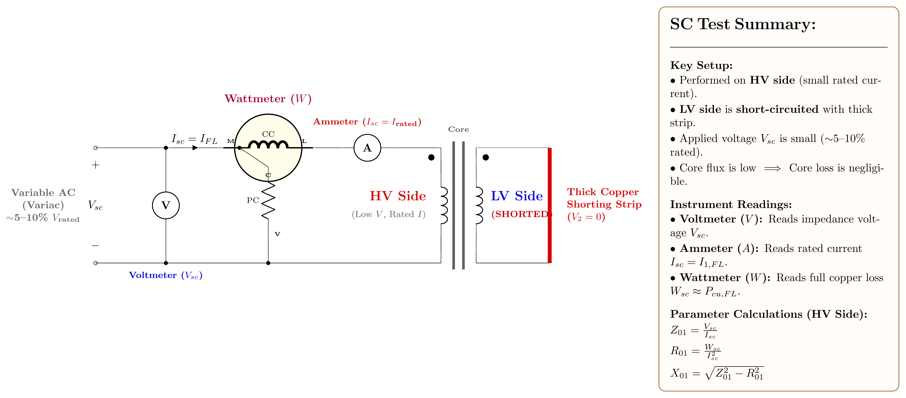
The Open-Circuit (OC) and Short-Circuit (SC) tests determine all equivalent circuit parameters and losses using only a tiny fraction of rated power (typically 2% to 5%):

• OC Test (Core Loss Specialist): Conducted at rated voltage on the LV side with HV open. Because secondary current is zero, primary winding copper loss is negligible ($I_0^2{R}_1\approx 0$). The input wattmeter measures strictly core loss ($P_c=P_h+P_e$) at rated flux density, extracting shunt parameters $R_c$ and $X_m$.
• SC Test (Copper Loss Specialist): Conducted at rated current on the HV side with LV short-circuited. Because the applied voltage is tiny (only 5% to 10% of rated), the core flux is proportionally tiny ($\Phi \propto V_{sc}$), making core loss practically zero ($P_c\propto V_{sc}^2\approx 1\%\text{ of rated}$). The input wattmeter measures strictly full-load copper loss, extracting series parameters $R_{01}$ and $X_{01}$.
• Predictive Power: Once $R_c,X_m,R_{01},X_{01}$ are known, efficiency and voltage regulation can be mathematically computed for any arbitrary load fraction $x$ and any power factor $\cos \varphi$ with high precision without ever connecting a physical load.

---

Q3(b): 20 kVA, 2000/400V OC/SC Numerical Deconstructed

Problem Statement Breakdown:

• Rating: $S=20\text{ kVA}=20,000\text{ VA}$
• Voltage rating: $V_1/V_2=2000/400\text{ V}$
• Turns ratio: $a=\frac{N_1}{N_2}=\frac{2000}{400}=5$
• Rated HV current: $I_{1,\text{rated}}=\frac{20,000}{2000}=10\text{ A}$
• Rated LV current: $I_{2,\text{rated}}=\frac{20,000}{400}=50\text{ A}$

1. OC Test Interpretation (conducted on LV side, 400 V):

Instruments read: $V_0=400\text{ V}$, $I_0=1.5\text{ A}$, $W_0=160\text{ W}$. Since the test was conducted on the LV side, these readings yield LV-side core parameters:

• No-load power factor: $$\cos {\varphi }_0=\frac{W_0}{V_0{I}_0}=\frac{160}{400\times 1.5}=\frac{160}{600}=0.2667$$
• Core-loss and magnetizing currents (LV side): $$I_c=I_0\cos {\varphi }_0=1.5\times 0.2667=0.400\text{ A}$$ $$I_m=\sqrt{I_0^2-I_c^2}=\sqrt{1.5^2-0.4^2}=\sqrt{2.25-0.16}=\sqrt{2.09}=1.4457\text{ A}$$
• Shunt parameters referred to LV side: $$R_{c,\text{LV}}=\frac{V_0}{I_c}=\frac{400}{0.400}=1000\Omega$$ $$X_{m,\text{LV}}=\frac{V_0}{I_m}=\frac{400}{1.4457}=276.68\Omega$$
• Referring to HV side ($\times a^2=5^2=25$): $$R_{c1}=a^2{R}_{c,\text{LV}}=25\times 1000=\boxed{25,000\Omega }$$ $$X_{m1}=a^2{X}_{m,\text{LV}}=25\times 276.68=\boxed{6,917\Omega \approx 6,920\Omega }$$

(Sanity Check: Shunt core resistance and reactance referred to HV are in thousands of ohms, which makes physical sense because they draw only a tiny fraction of an ampere from the 2000 V primary.)

2. SC Test Interpretation (conducted on HV side):

Instruments read: $V_{sc}=60\text{ V}$, $I_{sc}=10\text{ A}$ (rated HV current), $W_{sc}=300\text{ W}$. Since meters are on the HV side, parameters are obtained directly referred to the primary:

• Total equivalent series resistance: $$R_{01}=\frac{W_{sc}}{I_{sc}^2}=\frac{300}{10^2}=\boxed{3.0\Omega }$$
• Total equivalent series impedance: $$Z_{01}=\frac{V_{sc}}{I_{sc}}=\frac{60}{10}=6.0\Omega$$
• Total equivalent series leakage reactance: $$X_{01}=\sqrt{Z_{01}^2-R_{01}^2}=\sqrt{6.0^2-3.0^2}=\sqrt{36-9}=\sqrt{27}=\boxed{5.196\Omega }$$

3. Efficiency at Full Load, 0.8 PF Lagging:

• Useful output active power: $$P_{\text{out}}=S\cos \varphi =20,000\times 0.8=16,000\text{ W}$$
• Total losses:
  • Iron loss (from OC test, constant): $P_i=160\text{ W}$
  • Full-load copper loss (from SC test at rated current): $P_{Cu}=300\text{ W}$ $$P_{\text{loss}}=160+300=460\text{ W}$$
• Efficiency: $$\eta =\frac{P_{\text{out}}}{P_{\text{out}}+P_{\text{loss}}}=\frac{16,000}{16,000+460}=\frac{16,000}{16,460}=\boxed{97.20\%}$$

4. Voltage Regulation at Full Load, 0.8 PF Lagging:

For lagging power factor ($\cos \varphi =0.8⟹\sin \varphi =0.6$): $$\Delta V_1=I_1(R_{01}\cos \varphi +X_{01}\sin \varphi )$$ $$\Delta V_1=10\times (3.0\times 0.8+5.196\times 0.6)=10\times (2.40+3.118)=10\times 5.518=55.18\text{ V}$$ $$\text{VR\%}=\frac{\Delta V_1}{V_1}\times 100=\frac{55.18}{2000}\times 100=\boxed{2.76\%}$$

---

Question 4

Q4(a): Derivation of the Transformer EMF Equation

For the comprehensive derivation, physical picture, and design implications see T-01: EMF Equation: $E=4.44fN{\Phi }_m$.

Key Physical Takeaways:

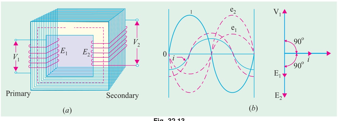
1. Why the factor is 4.44 and not 4: In one cycle, the alternating flux changes from $0\to +{\Phi }_m\to 0\to -{\Phi }_m\to 0$, traversing a total flux change of $4{\Phi }_m$ in time $T=1/f$. Thus, the average EMF per turn is strictly $4f{\Phi }_m$. But AC equipment works on RMS (heating/effective) value. For a sinusoidal waveform, the form factor is $K_f=\frac{\text{RMS}}{\text{Average}}=\frac{\pi }{2\sqrt{2}}\approx 1.1107$. Multiplying average by form factor gives: $$\text{RMS EMF per turn}=1.1107\times 4f{\Phi }_m=4.4428f{\Phi }_m\approx 4.44f{\Phi }_m$$
2. Phase Relationship: Because differentiation of $\sin (\omega t)$ yields $\cos (\omega t)=\sin (\omega t+90°)$, with the Lenz's law minus sign, the induced EMF lags the mutual flux by 90°.

---

Q4(b): Turns Calculation and Core Magnetic Design ($6.6\text{ kV}/400\text{ V}$)

Problem Data:

• Frequency $f=50\text{ Hz}$
• Primary voltage $V_1=6600\text{ V}$, Secondary voltage $V_2=400\text{ V}$
• Gross core area $A=25{\text{ cm}}^2=25\times 10^{-4}{\text{ m}}^2=0.0025{\text{ m}}^2$
• Maximum allowable flux density $B_m=1.2\text{ T}$

Step-by-step physical solution:

1. Core Flux Capacity: The maximum magnetic flux that the iron core can support before saturating is: $${\Phi }_m=B_m\times A=1.2\times (25\times 10^{-4})=3.0\times 10^{-3}\text{ Wb}=3\text{ mWb}$$
2. Volts-per-Turn ($E_t$): Every single loop of wire linked by this core flux has an induced RMS voltage of: $$E_t=4.44f{\Phi }_m=4.44\times 50\times (3\times 10^{-3})=0.666\text{ Volts/turn}$$ Design Insight: Volts-per-turn is the fundamental magnetic constant of a given core. Both primary and secondary windings must adhere to this exact same ratio.
3. Primary Turns ($N_1$): $$N_1=\frac{E_1}{E_t}=\frac{6600}{0.666}=\boxed{9,910\text{ turns}}$$
4. Secondary Turns ($N_2$): $$N_2=\frac{E_2}{E_t}=\frac{400}{0.666}=\boxed{600\text{ turns}}$$
5. Check: $$\frac{N_1}{N_2}=\frac{9910}{600}=16.517\approx \frac{6600}{400}=16.50✓$$

---

Q4(c): Equivalent Circuit Referred to Primary Side

See detailed circuit transformation steps in 2020 Explanation: Q1(a).

The physical philosophy of "Referring"

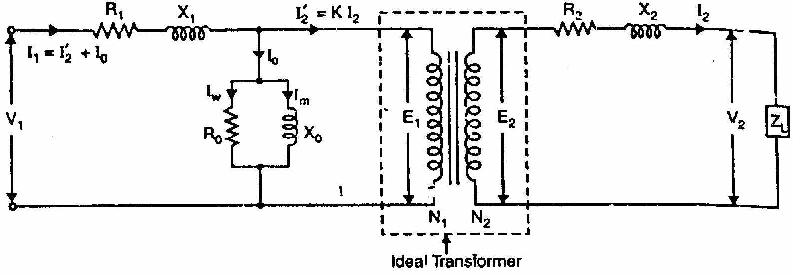
A transformer contains two galvanically isolated circuits separated by an air-gap/core boundary. To solve this using standard circuit analysis techniques (Kirchhoff's laws, Thevenin's theorem), we transfer all secondary impedances and voltages across the magnetic barrier into equivalent primary quantities:

• Impedance Scaling by $a^2$: Since secondary voltage scales by $a=N_1/N_2$ and current scales by $1/a$, secondary impedance scales by voltage-to-current ratio: $$Z_2^{\prime }=\frac{V_2^{\prime }}{I_2^{\prime }}=\frac{a{V}_2}{I_2/a}=a^2\frac{V_2}{I_2}=a^2{Z}_2$$ Therefore: $R_2^{\prime }=a^2{R}_2$ and $X_2^{\prime }=a^2{X}_2$.
• Combining Series Branches: The total primary-referred winding resistance is $R_{01}=R_1+R_2^{\prime }$, and total leakage reactance is $X_{01}=X_1+X_2^{\prime }$.
• Why the Approximate Circuit is Justified: In the exact circuit, the magnetizing branch ($R_c\Vert j{X}_m$) is placed between primary impedance ($R_1+j{X}_1$) and secondary impedance ($R_2^{\prime }+j{X}_2^{\prime }$). In the approximate circuit, this parallel branch is shifted all the way to the input terminals. Physical justification: Because no-load current $I_0$ is very small (2–5% of rated), the voltage drop across $R_1+j{X}_1$ caused by $I_0$ is less than 0.5% of $V_1$. Shifting the shunt branch introduces negligible calculation error while turning a two-loop circuit into a simple single-loop series-parallel network.

---

Question 5

Q5(a): Rotating Magnetic Field (RMF) Proof and Physical Meaning

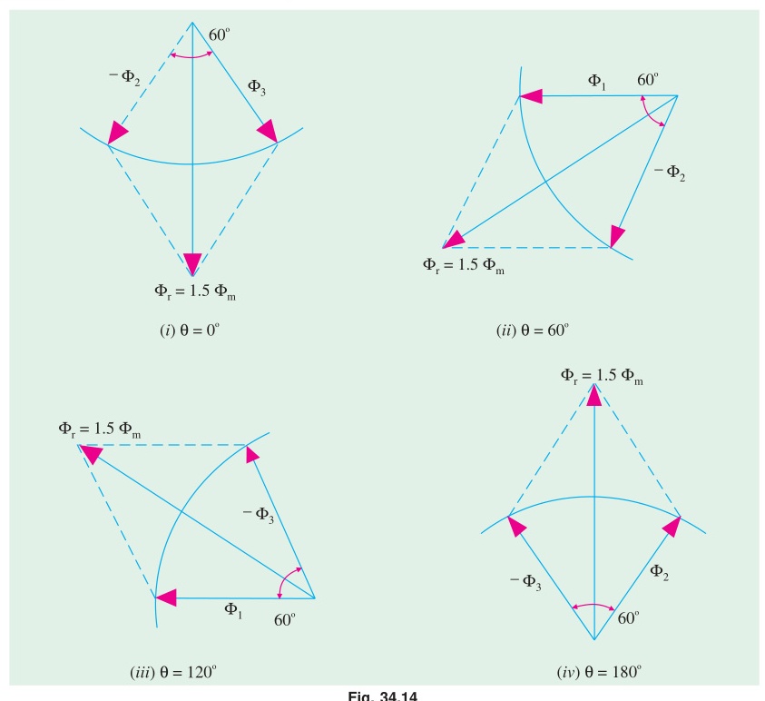
The physical magic of RMF

A single-phase winding produces only a pulsating field that grows, collapses, reverses, and dies along a fixed spatial axis. It does not rotate.

When three identical stator windings are placed 120° apart in space around the cylindrical stator periphery and energized by balanced 3-phase currents displaced by 120° in time, their individual pulsating flux waves superimpose to produce a single resultant magnetic flux wave.

Mathematical verification:

Let the three pulsating fluxes along their respective space axes (0°, 120°, 240°) be: $${\Phi }_R={\Phi }_m\sin \omega t,{\Phi }_Y={\Phi }_m\sin (\omega t-120°),{\Phi }_B={\Phi }_m\sin (\omega t+120°)$$ Resolving along horizontal ($X$) and vertical ($Y$) axes: $${\Phi }_x=\frac{3}{2}{\Phi }_m\sin \omega t,{\Phi }_y=-\frac{3}{2}{\Phi }_m\cos \omega t$$ The resultant magnitude: $${\Phi }_r=\sqrt{{\Phi }_x^2+{\Phi }_y^2}=\sqrt{{\left(\frac{3}{2}{\Phi }_m\right)}^2({\sin }^2\omega t+{\cos }^2\omega t)}=\boxed{1.5{\Phi }_m=\text{constant}}$$ The spatial angle of the resultant vector: $$\theta ={\tan }^{-1}\left(\frac{{\Phi }_y}{{\Phi }_x}\right)={\tan }^{-1}\left(\frac{-\cos \omega t}{\sin \omega t}\right)=\omega t-90°$$ The angular velocity of rotation is $\frac{d\theta }{dt}=\omega =2\pi f$ electrical radians per second, corresponding to synchronous speed $N_s=\frac{120f}{P}$ rpm.

Why $1.5{\Phi }_m$ and not $3{\Phi }_m$? Because the three phases never peak at the same moment in time. When phase $R$ is at peak (${\Phi }_m$), phases $Y$ and $B$ are both at $-0.5{\Phi }_m$. Vector addition of these three spatial vectors yields $1.0{\Phi }_m-(-0.5{\Phi }_m)=1.5{\Phi }_m$.

---

Q5(b): Power Flow Ratios in an Induction Motor: $(1-s):s:1$

For full derivation and power-flow tree diagram see IM-01: Air-Gap Power Ratios.

Physical mechanism of power transfer across the air gap:

1. Air-Gap Power ($P_g$): Electrical power transferred across the air gap from stator to rotor via the rotating magnetic field. Across the equivalent circuit rotor branch, it is dissipated in the equivalent resistance $R_2/s$: $$P_g=3I_2^2\frac{R_2}{s}$$
2. Rotor Ohmic Loss ($P_{r,Cu}$): The physical heat lost in the rotor conductors due to circulating rotor current: $$P_{r,Cu}=3I_2^2{R}_2=s\left(3I_2^2\frac{R_2}{s}\right)=s{P}_g$$
3. Internal Mechanical Power Developed ($P_m$): The net electromechanical power converted into rotational mechanical drive: $$P_m=P_g-P_{r,Cu}=P_g-s{P}_g=(1-s)P_g$$
4. The Fundamental Ratio: $$P_m:P_{r,Cu}:P_g=(1-s)P_g:s{P}_g:P_g=\boxed{(1-s):s:1}$$

Crucial Engineering Insight: The rotor electrical efficiency is $\frac{P_m}{P_g}=(1-s)$. To operate an induction motor with high efficiency, slip $s$ must be kept small (typically 2% to 5% at full load). High slip directly burns energy as rotor heat.

---

Question 6

Q6(a): Maximum Torque Derivation and Independence of $R_2$

For full mathematical derivation see IM-02: Maximum Torque is Independent of Rotor Resistance.

The physical balance at maximum torque

The internal torque of an induction motor is given by: $$T=\frac{ks{E}_2^2{R}_2}{R_2^2+s^2{X}_2^2}$$ Differentiating with respect to slip $s$ yields the maximum torque condition: $$s_{mT}=\frac{R_2}{X_2}$$ Substituting this condition back into the torque equation: $$T_{\max }=\frac{k{E}_2^2}{2X_2}$$

Why does rotor resistance $R_2$ disappear from $T_{\max }$?

This seems counterintuitive at first: if you increase rotor resistance, doesn't that waste more power and reduce torque? The answer lies in the competition between rotor current magnitude and rotor power factor:

• Torque is proportional to flux, current, and rotor power factor: $T\propto {\Phi }_m{I}_2\cos {\theta }_2$.
• At breakdown torque ($s_{mT}=R_2/X_2$), the rotor inductive reactance $s{X}_2$ equals the rotor resistance $R_2$.
• At this exact point, the rotor power factor angle is always ${\theta }_2={\tan }^{-1}(s{X}_2/R_2)={\tan }^{-1}(1)=45°$, so $\cos {\theta }_2=\cos 45°=1/\sqrt{2}$ regardless of what $R_2$ is!
• Increasing $R_2$ simply requires a higher slip $s$ to make $s{X}_2$ catch up to $R_2$. The peak torque itself is completely unaltered; it is merely shifted to a lower operating speed.

---

Q6(b): 6-Pole, 400V, 50 Hz IM Numerical Problem Step-by-Step

Problem Parameters:

• Poles $P=6$, Frequency $f=50\text{ Hz}$, Connection: Star (Wye)
• Line Voltage $V_L=400\text{ V}⟹V_{\varphi }=\frac{400}{\sqrt{3}}\approx 231.0\text{ V}$
• Referred rotor resistance $R_2^{\prime }=0.5\Omega$, standstill reactance $X_2^{\prime }=2.0\Omega$
• Full-load slip $s=0.04$ (4%)
• Mechanical losses (friction & windage) $P_{\text{mech}}=500\text{ W}$

1. Speeds and Constants:

• Synchronous speed: $$N_s=\frac{120\times 50}{6}=1000\text{ rpm}⟹{\omega }_s=\frac{2\pi \times 1000}{60}=104.72\text{ rad/s}$$
• Torque constant: $$k=\frac{3}{{\omega }_s}=\frac{3}{104.72}=0.028648\text{ N-m}\cdot \text{s/W}$$

2. Starting Torque ($s=1$):

At standstill ($s=1$), rotor reactance is at its highest ($X_2=2.0\Omega \gg R_2=0.5\Omega$): $$T_{st}=\frac{k\cdot (1)\cdot E_2^2\cdot R_2}{R_2^2+(1{)}^2{X}_2^2}=\frac{0.028648\times (231{)}^2\times 0.5}{0.5^2+2.0^2}=\frac{0.028648\times 53361\times 0.5}{0.25+4.0}=\frac{764.32}{4.25}=\boxed{179.8\text{ N-m}}$$

3. Full-Load Running Torque ($s=0.04$):

At running speed, rotor reactance is throttled by slip ($s{X}_2=0.04\times 2.0=0.08\Omega \ll R_2=0.5\Omega$): $$T_{FL}=\frac{k\cdot s\cdot E_2^2\cdot R_2}{R_2^2+s^2{X}_2^2}=\frac{0.028648\times 0.04\times 53361\times 0.5}{0.5^2+(0.04\times 2.0{)}^2}=\frac{30.573}{0.25+0.0064}=\frac{30.573}{0.2564}=\boxed{119.2\text{ N-m}}$$

4. Maximum (Pull-Out) Torque:

• Slip at max torque: $s_{mT}=\frac{R_2}{X_2}=\frac{0.5}{2.0}=0.25$ (25% slip)
• Breakdown torque: $$T_{\max }=\frac{k{E}_2^2}{2X_2}=\frac{0.028648\times 53361}{2\times 2.0}=\frac{1528.69}{4.0}=\boxed{382.2\text{ N-m}}$$

(Sanity Check: Notice that $T_{\max }=382.2\text{ N-m}>T_{st}=179.8\text{ N-m}>T_{FL}=119.2\text{ N-m}$. Maximum torque is over 3.2 times full-load torque, typical for an industrial squirrel-cage induction motor).

5. Power Balance and Full-Load Efficiency:

• Air-gap power at full load: $$P_g=T_{FL}\times {\omega }_s=119.2\times 104.72=12,483\text{ W}$$
• Rotor copper loss: $$P_{r,Cu}=s{P}_g=0.04\times 12,483=499.3\text{ W}$$
• Developed mechanical power: $$P_m=(1-s)P_g=0.96\times 12,483=11,984\text{ W}$$
• Net shaft output power: $$P_{\text{shaft}}=P_m-P_{\text{mech}}=11,984-500=11,484\text{ W}\approx 11.48\text{ kW}$$
• Stator losses estimation (assuming typical stator core + copper loss $\approx 500\text{ W}$): $$P_{\text{in}}=P_g+P_{\text{stator losses}}=12,483+500=12,983\text{ W}$$ $$\eta =\frac{P_{\text{shaft}}}{P_{\text{in}}}\times 100=\frac{11,484}{12,983}\times 100=\boxed{88.5\%}$$

---

Question 7

Q7(a): Induction Motor Testing and Parameter Extraction

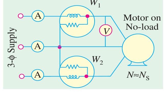
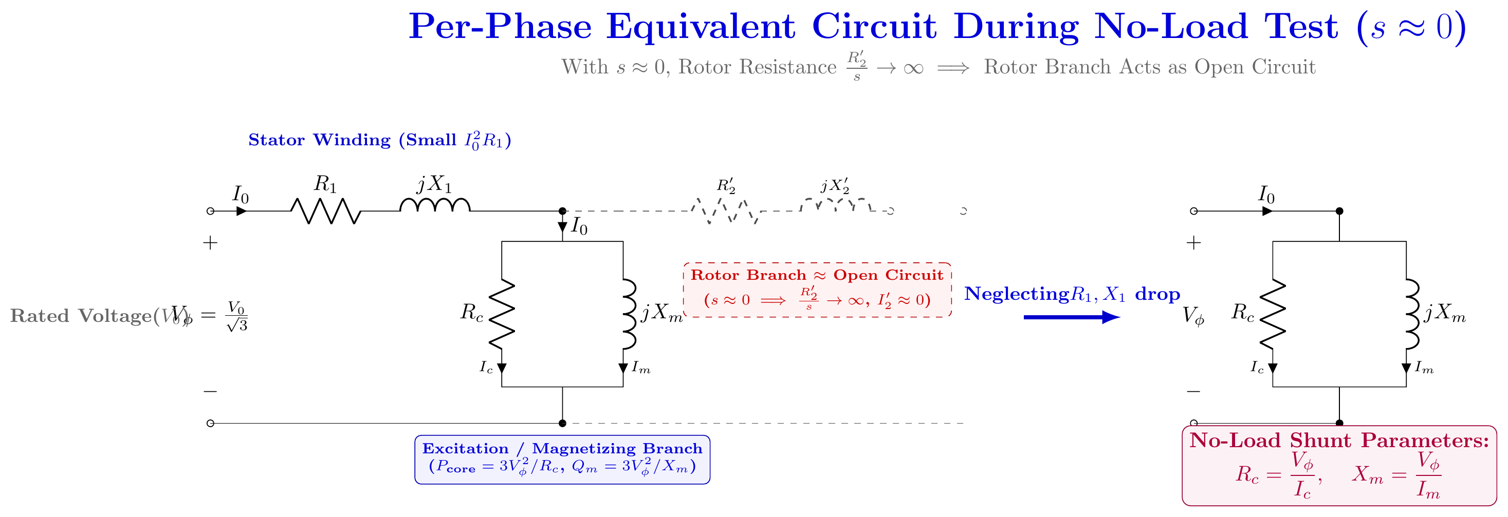
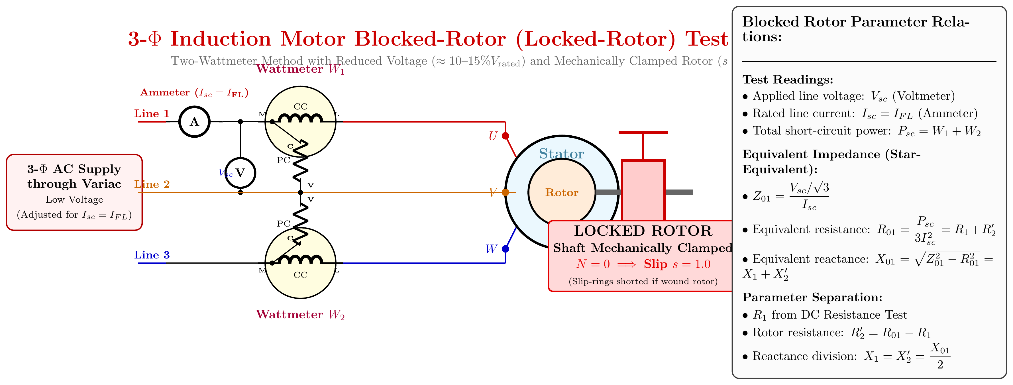
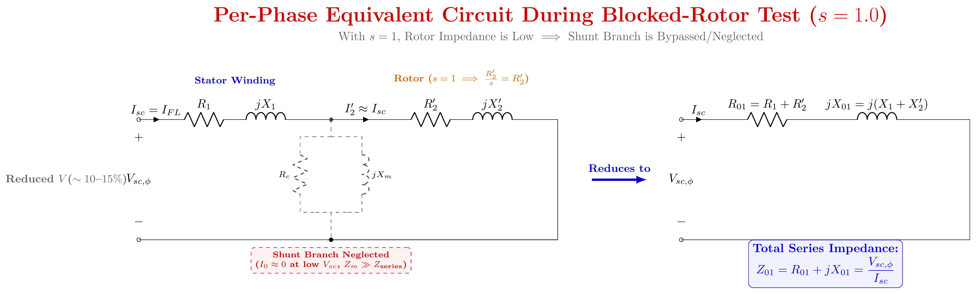
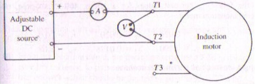
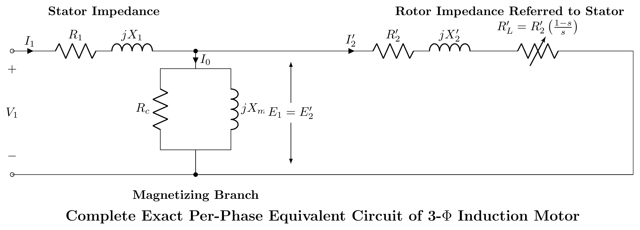
For complete detailed procedure see IM-04: Blocked Rotor Test: Full Procedure and Why It's Needed.

Physical meaning of the parameter extraction:

1. Why No-Load Slip is Virtually Zero ($s\approx 0$): With no mechanical shaft resistance, rotor friction is overcome by minimal torque. Rotor accelerates to $N\approx N_s$. Because $s\to 0$, the fictitious load resistance representing mechanical load $\frac{R_2^{\prime }}{s}(1-s)\to \infty$. The rotor branch becomes an open circuit! Therefore, the motor draws almost entirely magnetizing current $I_0$ to excite the air gap, exposing $R_c$ and $X_m$.
2. Why Blocked-Rotor Test Uses Low Voltage (~15%): With the shaft clamped, slip is $s=1.0$, making effective load resistance zero ($\frac{1-s}{s}=0$). If full rated voltage were applied, an extreme locked-rotor current (600% to 800% of rated) would destroy the winding insulation within seconds. By dialing down the voltage to ~15%, full rated current is safely circulated, and core loss drops to virtually zero ($P_{\text{core}}\propto V^2\approx (0.15{)}^2\approx 2\%$). The wattmeter measures strictly the copper losses of stator and rotor ($R_{01}=R_1+R_2^{\prime }$).
3. The DC Test Necessity: The blocked rotor test only provides the sum $R_{01}=R_1+R_2^{\prime }$. A DC test across two stator terminals gives $R_{1,DC}$, which is multiplied by a skin-effect factor (1.25 for 50 Hz) to give AC resistance $R_1$. Subtracting $R_1$ from $R_{01}$ isolates $R_2^{\prime }$.

---

Q7(b): Effect of Rotor Resistance on Torque-Speed Characteristic

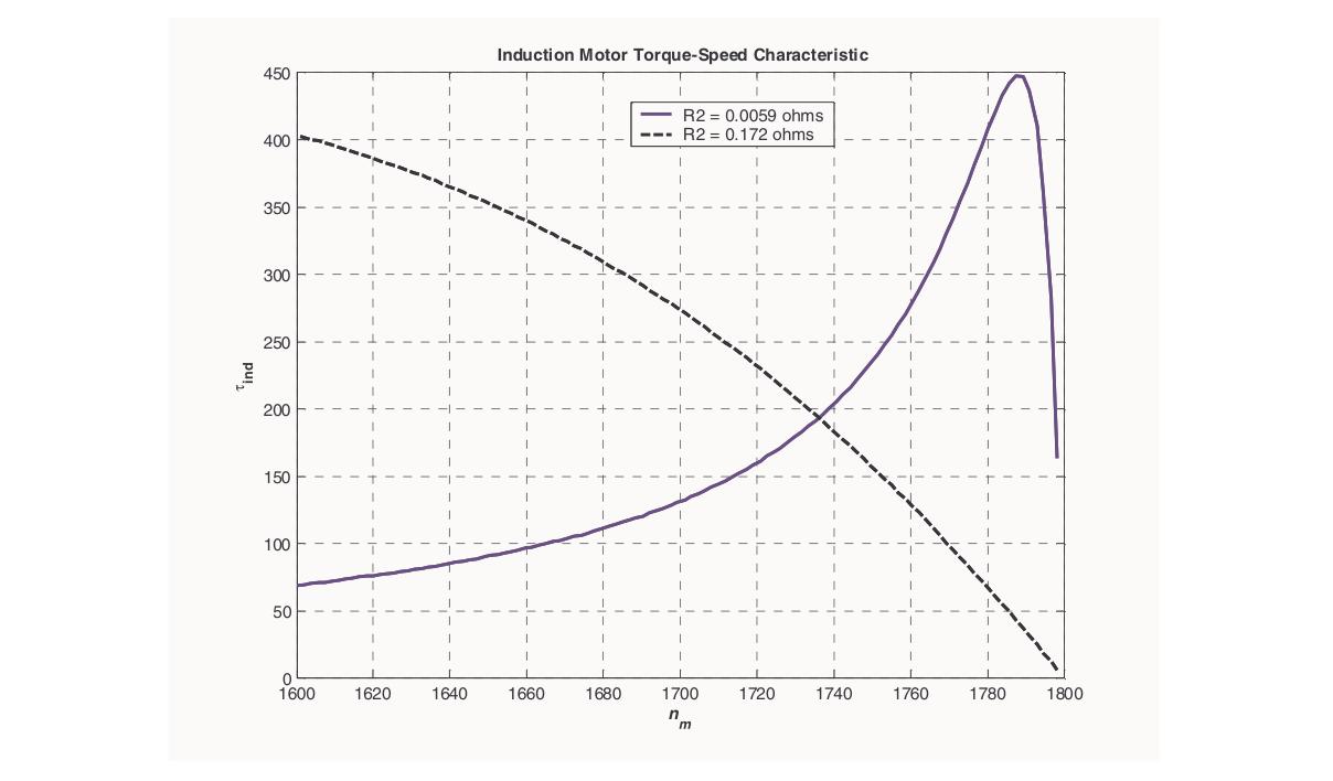
The engineering tradeoff: Starting vs Running

The torque-speed curve demonstrates one of the most critical compromises in electrical machine design:

1. Starting Region ($s=1.0$): At starting, standstill reactance dominates ($X_2\gg R_2$). A standard low-resistance squirrel-cage rotor produces poor starting torque with a terrible lagging power factor ($\cos {\theta }_2\approx 0.2$).
   • By adding external resistance $R_{ext}$ into the rotor circuit (possible in wound-rotor motors via slip rings), total rotor resistance increases to $R_{2,\text{total}}=R_2+R_{ext}$.
   • The starting torque increases dramatically: if $R_{2,\text{total}}$ is designed to equal $X_2$, the motor develops its absolute maximum possible torque right at standstill ($T_{st}=T_{\max }$).
   • Starting current is simultaneously reduced because total impedance $Z=\sqrt{R_{2,\text{total}}^2+X_2^2}$ is larger.
2. Running Region (Low Slip): Once the motor accelerates up to rated speed, high rotor resistance becomes an enormous liability!
   • Full-load slip would have to be very high to generate operating torque ($s\propto R_2$).
   • Since rotor copper loss is $P_{r,Cu}=s{P}_g$, running efficiency $\eta \approx (1-s)$ drops drastically, and the motor overheats.
3. The Wound-Rotor Solution: Slip-ring motors insert external resistance during start-up to achieve maximum starting torque with gentle starting current, and then progressively cut out the external resistors as speed picks up, running at full speed with short-circuited slip rings for maximum efficiency.

---

Question 8

Q8(a): Single-Phase Induction Motor and Double Revolving Field Theory

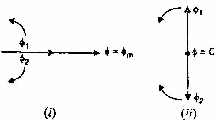
For full mathematical formulation see IM-03: Single-Phase Induction Motor: Double Revolving Field Theory.

Why a 1-phase IM cannot start itself:

• A single stator winding produces a pulsating stationary flux: $\Phi (t)={\Phi }_m\sin \omega t$.
• By Ferraris' theorem, this decomposes into two equal and opposite rotating magnetic fields:
  • Forward field of strength $\frac{{\Phi }_m}{2}$ rotating clockwise at $+N_s$.
  • Backward field of strength $\frac{{\Phi }_m}{2}$ rotating counter-clockwise at $-N_s$.
• At standstill ($N=0$), both fields see the exact same slip $s_f=s_b=1.0$. The forward torque $T_f$ and backward torque $T_b$ are completely identical in magnitude and opposite in direction: $$T_{\text{net}}=T_f-T_b=0$$ The rotor experiences severe vibrational humming, but zero net starting torque.

Why it continues running once started:

If given an initial mechanical push in the forward direction ($N>0$):

• Forward slip decreases: $s_f=\frac{N_s-N}{N_s}\ll 1$ (e.g., $0.05$).
• Backward slip increases: $s_b=\frac{N_s-(-N)}{N_s}=2-s_f\approx 1.95$.
• At small slip $s_f=0.05$, the forward rotor branch has high effective impedance and develops large forward torque $T_f$. At $s_b\approx 1.95$, the backward rotor branch appears virtually short-circuited, producing high rotor copper loss and negligible backward torque $T_b$.
• Therefore, $T_f\gg T_b$, producing a strong positive net torque that accelerates and sustains motor rotation in the direction of the initial push.

---

Q8(b): Two Practical Types of Single-Phase Induction Motors

To make a single-phase induction motor self-starting, we must artificially convert the pulsating single-phase field into an unbalanced rotating magnetic field during starting.

1. Capacitor-Start, Capacitor-Run Motor (Two-Value Capacitor Motor)

Physical Mechanism:

This motor uses two stator windings placed 90° apart in space: the Main Winding (heavy gauge, many turns, high inductance) and the Auxiliary Winding (finer wire, fewer turns) in series with capacitors.

• Starting Phase: A large electrolytic starting capacitor $C_s$ (~200–400 $\mu$F) is connected in parallel with the run capacitor $C_r$. The large net capacitance causes the auxiliary winding current $I_A$ to lead the supply voltage by ~40°, while main winding current $I_M$ lags by ~50°. The resulting phase displacement between the two currents is: $$\alpha ={\varphi }_M+{\varphi }_A\approx 50°+40°=90°$$ With two windings 90° apart in space carrying currents 90° apart in time, a nearly perfect circular rotating magnetic field is established, producing an exceptional starting torque (250% to 350% of full-load torque).
• Running Phase: Once the rotor reaches ~75% synchronous speed, a centrifugal switch disconnects the short-time-rated electrolytic capacitor $C_s$. The smaller continuous-rated AC oil-filled capacitor $C_r$ (~10–30 $\mu$F) remains in circuit.
• Why keep $C_r$ during running? In a standard split-phase motor, the auxiliary winding is cut out completely, turning the running motor back into a noisy single-phase machine. In the two-value motor, keeping $C_r$ maintains a balanced two-phase rotating field at full load. This eliminates pulsating torque, produces whisper-quiet running, dramatically improves the motor power factor ($\approx 0.95$), and raises overall efficiency.
• Typical Applications: Heavy-duty continuous-load appliances: refrigerator compressors, water pumps, air conditioners, conveyor drives.

---

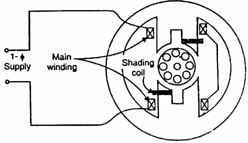
2. Shaded-Pole Motor

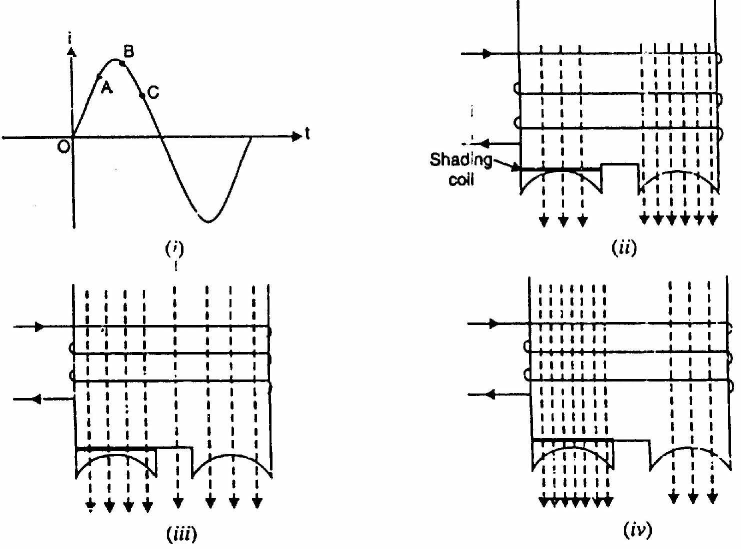
Physical Mechanism:

The shaded-pole motor is the simplest, most rugged, and cheapest of all single-phase motors. It requires no auxiliary winding, no capacitors, and no centrifugal switch.

• Construction: It uses salient (projecting) stator poles. A small portion (typically 1/3) of each pole face is notched and encircled by a heavy, closed single-turn copper ring known as the shading band or shading coil.
• The Sweeping Flux Action:
  1. Flux Rising: When alternating current starts to rise from zero in the main field coil, core flux begins to grow. The changing flux induces a strong circulating current in the shorted copper shading band. By Lenz's law, this induced current creates an opposing MMF that delays flux buildup in the shaded portion. The flux is therefore forced to crowd into the unshaded portion of the pole.
  2. Flux Peak: Near the crest of the AC sine wave, the rate of flux change is zero ($d\Phi /dt=0$). Induced shading current dies away, and flux distributes uniformly across both unshaded and shaded portions.
  3. Flux Falling: As the main AC current declines towards zero, the decaying flux induces a shading current that tries to sustain the dying flux (Lenz's law). The flux now collapses rapidly in the unshaded section while persisting in the shaded section.
• Net Result: The peak magnetic flux shifts progressively across the pole face from the unshaded segment toward the shaded segment. This sweeping action creates an equivalent moving field that drags the squirrel-cage rotor along in the direction from unshaded $\to$ shaded pole.
• Trade-offs:
  • Starting torque: Very weak (40% to 60% of full load).
  • Efficiency: Very poor (typically 15% to 35%), because the shorted copper band continuously dissipates $I^{2}R$ heat throughout normal operation.
  • Direction: Strictly unidirectional (cannot be reversed electrically).
  • Advantages: Extremely low cost, zero maintenance, indefinite lifespan.
• Typical Applications: Low-torque, low-power small loads where efficiency is secondary to reliability and cost: small desk fans, PC chassis cooling fans, microwave oven turntables, hair dryers.

---

Source: PrevYearQuestions/2024.md

---

← 2023 Answer | 🏠 Index | 2018–2024 Repeated Questions →