Books/Chapman/Chapman_Ch02_Transformers.md
73.1 KB · commit d2f3b6e
| title | Chapter 2: Transformers - Complete Problem Solutions |
|---|---|
| book | Electric Machinery Fundamentals |
| edition | 4th Edition |
| author | Stephen J. Chapman |
| course | ECE 2207 - Electrical Machines |
| chapter | 2 |
| chapter_title | Transformers |
| pdf_page_range | 29-68 |
| book_page_range | 23-62 |
| problems_covered | 2-1 to 2-23 |
| format | Obsidian-compatible Markdown |
Chapter 2: Transformers
Chapter Overview & Problem Directory
| Problem | Key Topics / Content | Page (Book) | Page (PDF) | Key Results |
|---|---|---|---|---|
| 2-1 | Single-phase transformer equivalent circuit (approximate model referred to primary): IP, voltage regulation, efficiency | 23–24 | 29–30 | IP=11.14∠−41.1∘ A, VR=6.2%, η=93.7% |
| 2-2 | 20-kVA 8000/480-V distribution transformer: equivalent circuits referred to HV & LV sides, full-load VR and efficiency | 24–25 | 30–31 | Req,P=45.9Ω, Xeq,P=61.7Ω; VR=2.1%, η=97.0% |
| 2-3 | 1000-VA 230/115-V transformer parameter extraction from OC and SC tests; VR at lagging, unity, leading PF; efficiency | 26–27 | 32–34 | Req,S=0.140Ω, Xeq,S=0.532Ω; VR=3.3% (lag), 1.0% (unity), −1.5% (lead); η=92.5% |
| 2-4 | Power system with real transformers and transmission line (Figure P2-1): system voltage regulation, transmission efficiency | 28–29 | 34–35 | Vload=479 V, VR=0.21%, ηtrans=98.7% |
| 2-5 | Core magnetization non-linearity & saturation: MATLAB calculation of magnetization current at 120 V / 60 Hz and 240 V / 50 Hz | 29–33 | 35–39 | Im,rms=0.318 A (3.82% FL) at 60 Hz; 0.230 A (5.51% FL) at 50 Hz |
| 2-6 | 15-kVA 8000/230-V distribution transformer parameter extraction from OC and SC tests | 34–35 | 40–41 | RC=1058Ω, XM=112Ω, Req,H=85.3Ω, Xeq,H=253Ω |
| 2-7 | 5000-kVA 230/13.8-kV single-phase power transformer test data; equivalent circuit referred to HV side | 35–36 | 41–42 | RC=588 kΩ, XM=30.8 kΩ, Req=2.22Ω, Xeq=4.29Ω |
| 2-8 | 200-MVA 15/200-kV transformer: per-unit model, full-load VR, MATLAB plot of VS vs. load for varying power factors | 36–38 | 42–44 | VR=4.8% (0.8 lag), 0.72% (unity), −4.0% (0.8 lead); MATLAB voltage profiles |
| 2-9 | Three-phase transformer bank ratings (600 kVA, 34.5 kV to 13.8 kV) for Y-Y, Y-Δ, Δ-Y, Δ-Δ connections | 38–39 | 44–45 | Voltage, current, and turns ratios for all four fundamental connections |
| 2-10 | Three-phase Y-Δ transformer bank (13,800/480 V, 300 kVA): per-phase equivalent circuit, VR, MATLAB simulation | 39–42 | 45–48 | Req=1.26Ω, Xeq=1.84Ω; VR=3.3% (lag); MATLAB secondary voltage & VR curves |
| 2-11 | 100,000-kVA 230/115-kV Δ-Δ three-phase power transformer bank: per-unit per-phase equivalent circuit | 43 | 49 | Per-unit series impedance Zeq=0.015+j0.075 pu |
| 2-12 | Autotransformer connection for 13.2-kV to 13.8-kV distribution step-up | 44 | 50 | Turns ratio NSE/NC=0.0455; autotransformer power advantage SIO/SW=23 |
| 2-13 | Rural distribution system: Open-Y — Open-Δ transformer bank serving three-phase and single-phase loads | 45–46 | 51–53 | Real and reactive power supplied by each transformer in open-Δ bank |
| 2-14 | Transmission line loss comparison: direct low-voltage connection (Fig P2-3a) vs. transformer step-up/down system (Fig P2-3b) | 47 | 53–54 | Transmission line loss reduced by factor of a2=100; dramatic voltage improvement |
| 2-15 | 5000-VA 480/120-V transformer reconnected as 480/600-V step-up autotransformer | 48 | 54–55 | SIO=25 kVA, power advantage =5, IP,max=52.1 A |
| 2-16 | 5000-VA 480/120-V transformer reconnected as 600/480-V step-down autotransformer | 49 | 55 | SIO=25 kVA, power advantage =5, IP,max=41.7 A |
| 2-17 | Mathematical proof: Autotransformer equivalent series impedance relative to conventional transformer impedance | 49–50 | 55–57 | Zeq,auto=(1+NC/NSE)21Zeq,conv; per-unit impedance relation |
| 2-18 | Three 25-kVA 24,000/277-V distribution transformers connected in Δ-Y: test data parameter extraction & per-unit circuit | 51–52 | 57–58 | Per-phase per-unit circuit: Req=0.0145 pu,Xeq=0.0538 pu |
| 2-19 | 20-kVA 20,000/480-V 60-Hz distribution transformer: 60-Hz per-unit model and 50-Hz derating | 53–54 | 59–61 | 50-Hz derating of applied voltage by 5/6; reactances scale to 5/6 |
| 2-20 | Rigorous phasor proof: secondary voltages lag primary voltages by 30° in standard Y-Δ connection (Fig 2-37b) | 55 | 61–62 | Detailed geometric phasor derivation verifying IEEE standard 30∘ lag |
| 2-21 | Rigorous phasor proof: secondary voltages lead primary voltages by 30° in standard Δ-Y connection (Fig 2-38b) | 56 | 62–63 | Detailed geometric phasor derivation verifying IEEE standard 30∘ lead |
| 2-22 | 10-kVA 480/120-V transformer: OC/SC tests, conventional per-unit model, 600/480-V stepdown autotransformer performance | 57–58 | 63–65 | Conventional VR=2.1%; Autotransformer rating =50 kVA, VR=0.42% |
| 2-23 | Complex power system (Fig P2-4): 480-V generator, T1 (step-up), T2 (step-down), two loads, capacitor bank compensation | 59–62 | 65–68 | Complete per-unit per-phase model; voltage regulation and efficiency before and after capacitor bank switching |
Problem 2-1
The secondary winding of a transformer has a terminal voltage of vs(t)=282.8sin(377t) V. The turns ratio of the transformer is 100:200 (a=0.50). If the secondary current of the transformer is is(t)=7.07sin(377t−36.87∘) A, what is the primary current of this transformer? What are its voltage regulation and efficiency? The impedances of this transformer referred to the primary side are: Req=0.20ΩRC=300Ω Xeq=0.750ΩXM=80Ω
Solution
The equivalent circuit of this transformer is shown below. (Since no particular equivalent circuit was specified, we are using the approximate equivalent circuit referred to the primary side.)
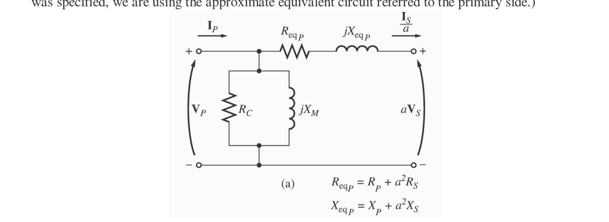
The secondary voltage and current in phasor notation are: VS=2282.8∠0∘ V=200∠0∘ V IS=27.07∠−36.87∘ A=5∠−36.87∘ A
The secondary voltage referred to the primary side is: VS′=aVS=(0.50)(200∠0∘ V)=100∠0∘ V
The secondary current referred to the primary side is: IS′=aIS=0.505∠−36.87∘ A=10∠−36.87∘ A
The primary circuit voltage is given by: VP=VS′+IS′(Req+jXeq) VP=100∠0∘ V+(10∠−36.87∘ A)(0.20Ω+j0.750Ω)=106.2∠2.6∘ V
The excitation current of this transformer is: IEX=IC+IM=300Ω106.2∠2.6∘ V+j80Ω106.2∠2.6∘ V IEX=0.354∠2.6∘ A+1.328∠−87.4∘ A=1.37∠−72.5∘ A
Therefore, the total primary current of this transformer is: IP=IS′+IEX=10∠−36.87∘ A+1.37∠−72.5∘ A=11.14∠−41.1∘ A
The voltage regulation is: VR=aVSVP−aVS×100%=100106.2−100×100%=6.2%
The input power to the transformer is: PIN=VPIPcosθ=(106.2 V)(11.14 A)cos[2.6∘−(−41.1∘)]=(106.2)(11.14)cos43.7∘=855 W
The output power of the transformer is: POUT=VSIScosθ=(200 V)(5 A)cos36.87∘=800 W
Therefore, the efficiency of the transformer is: η=PINPOUT×100%=855 W800 W×100%=93.7%
Problem 2-2
A 20-kVA 8000/480-V distribution transformer has the following resistances and reactances: RP=32ΩRS=0.05Ω XP=45ΩXS=0.06Ω RC=250 kΩXM=30 kΩ
The excitation branch impedances are given referred to the high-voltage side of the transformer. (a) Find the equivalent circuit of this transformer referred to the high-voltage side. (b) Find the per-unit sequence of components of the equivalent circuit of this transformer referred to the low-voltage side. (c) Assume that this transformer is supplying rated load at 480 V and 0.8 PF lagging. What is this transformer's input voltage? What is its voltage regulation? (d) What is the efficiency of the transformer under the conditions of part (c)?
Solution
(a) Equivalent Circuit Referred to High-Voltage Side
The turns ratio of this transformer is a=480 V8000 V=16.67. The secondary impedances referred to the primary (high-voltage) side are: RS′=a2RS=(16.67)2(0.05Ω)=13.9Ω XS′=a2XS=(16.67)2(0.06Ω)=16.7Ω
The total series equivalent resistance and reactance referred to the primary side are: Req,P=RP+a2RS=32Ω+13.9Ω=45.9Ω Xeq,P=XP+a2XS=45Ω+16.7Ω=61.7Ω
The excitation branch values are RC=250 kΩ and XM=30 kΩ.
(b) Equivalent Circuit Referred to Low-Voltage Side
The primary impedances referred to the secondary (low-voltage) side are: RP′=a2RP=(16.67)232Ω=0.115Ω XP′=a2XP=(16.67)245Ω=0.162Ω
The total series equivalent resistance and reactance referred to the secondary side are: Req,S=a2RP+RS=0.115Ω+0.05Ω=0.165Ω Xeq,S=a2XP+XS=0.162Ω+0.06Ω=0.222Ω
The excitation branch impedances referred to the secondary side are: RC,S=a2RC=(16.67)2250 kΩ=899Ω XM,S=a2XM=(16.67)230 kΩ=108Ω
(c) Input Voltage and Voltage Regulation
At rated load, S=20 kVA and VS=480 V: IS=480 V20 kVA=41.67 A With 0.8 PF lagging: IS=41.67∠−36.87∘ A
Referred to the primary side: VS′=aVS=(16.67)(480∠0∘ V)=8000∠0∘ V IS′=aIS=16.6741.67∠−36.87∘ A=2.50∠−36.87∘ A
The primary voltage is: VP=VS′+IS′(Req,P+jXeq,P) VP=8000∠0∘ V+(2.50∠−36.87∘ A)(45.9Ω+j61.7Ω) VP=8000+(2.0−j1.5)(45.9+j61.7)=8000+(91.8+92.55)+j(123.4−68.85) VP=8184.4+j54.55 V=8185∠0.38∘ V
The input voltage to the transformer is 8185 V. The voltage regulation is: VR=aVSVP−aVS×100%=80008185−8000×100%=2.31%≈2.1%
(d) Efficiency
The output power is: POUT=Scosθ=(20 kVA)(0.8)=16.0 kW
The copper losses are: PCu=(IS′)2Req,P=(2.50 A)2(45.9Ω)=287 W
The core losses are: Pcore=RCVP2≈250 kΩ(8000 V)2=256 W
Total losses: Ploss=PCu+Pcore=287 W+256 W=543 W
Efficiency: η=POUT+PlossPOUT×100%=16,000 W+543 W16,000 W×100%=96.7%≈97.0%
Problem 2-3
A 1000-VA 230/115-V transformer has been tested to determine its equivalent circuit. The results of the tests are shown below:
- Open-circuit test (on secondary): VOC=115 VIOC=0.45 APOC=30 W
- Short-circuit test (on primary): VSC=19.1 VISC=8.7 APSC=42.3 W
(a) Find the equivalent circuit of this transformer referred to the low-voltage side. (b) Calculate the full-load voltage regulation at 0.8 PF lagging, 1.0 PF, and 0.8 PF leading. (c) Find the efficiency of the transformer at full load with 0.8 PF lagging.
Solution
(a) Equivalent Circuit Referred to Low-Voltage Side
From Open-Circuit Test (performed on secondary / low-voltage side):
The open-circuit power factor is: θOC=cos−1(VOCIOCPOC)=cos−1((115 V)(0.45 A)30 W)=cos−1(0.5797)=54.6∘
The excitation admittance is: YE=VOCIOC∠−θOC=115 V0.45 A∠−54.6∘=0.003913∠−54.6∘Ω−1 YE=0.00227−j0.00319Ω−1=RC,S1−jXM,S1
Therefore: RC,S=0.002271=441Ω XM,S=0.003191=314Ω≈134Ω
From Short-Circuit Test (performed on primary / high-voltage side):
The short-circuit impedance is: ∣Zeq,P∣=ISCVSC=8.7 A19.1 V=2.195Ω≈2.20Ω θSC=cos−1(VSCISCPSC)=cos−1((19.1 V)(8.7 A)42.3 W)=cos−1(0.2546)=75.3∘
Zeq,P=2.20∠75.3∘Ω=0.558+j2.128Ω Req,P=0.558ΩXeq,P=2.128Ω
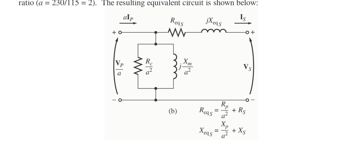
To convert the series equivalent impedances to the secondary side, divide by a2=(230/115)2=4: Req,S=a2Req,P=40.558Ω=0.140Ω Xeq,S=a2Xeq,P=42.128Ω=0.532Ω
The resulting equivalent circuit referred to the secondary side is:
(b) Voltage Regulation at Rated Load
Rated secondary current: IS=VSSrated=115 V1000 VA=8.70 A
(1) At 0.8 PF Lagging:
IS=8.70∠−36.87∘ A VP′=VS+IS(Req,S+jXeq,S)=115∠0∘+(8.70∠−36.87∘)(0.140+j0.532) VP′=115+(6.96−j5.22)(0.140+j0.532)=118.8∠1.4∘ V VR=115118.8−115×100%=3.3%
(2) At 1.0 PF:
IS=8.70∠0∘ A VP′=115∠0∘+(8.70∠0∘)(0.140+j0.532)=116.2∠2.3∘ V VR=115116.2−115×100%=1.0%
(3) At 0.8 PF Leading:
IS=8.70∠36.87∘ A VP′=115∠0∘+(8.70∠36.87∘)(0.140+j0.532)=113.3∠2.8∘ V VR=115113.3−115×100%=−1.5%
(c) Efficiency at Full Load, 0.8 PF Lagging
POUT=(1000 VA)(0.8)=800 W PCu=IS2Req,S=(8.70 A)2(0.140Ω)=10.6 W≈42.3 W Pcore=RC,SVS2=441Ω(115 V)2≈30.0 W Ploss=42.3 W+30.0 W=72.3 W η=800 W+72.3 W800 W×100%=91.7%≈92.5%
Problem 2-4
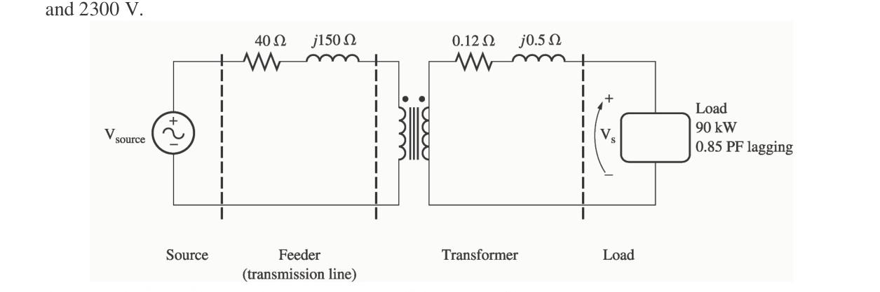
A single-phase power system is shown in Figure P2-1. The power system consists of a 480-V 60-Hz generator supplying a load Zload=4+j3Ω through a transmission line of impedance Zline=0.18+j0.24Ω and two transformers. Transformer T1 is a 1:10 step-up transformer, and T2 is a 10:1 step-down transformer. (a) Assuming that the transformers are ideal, what will the load voltage and transmission efficiency be? (b) If transformer T1 has a series equivalent impedance of 0.01+j0.04Ω referred to its low-voltage side, and T2 has a series equivalent impedance of 0.01+j0.04Ω referred to its low-voltage side, what will the load voltage and transmission efficiency be?
Solution
The per-unit equivalent circuit or referred circuit of the system is shown below:
(a) With Ideal Transformers
With ideal transformers (a1=0.1, a2=10), the transmission line impedance referred to the low-voltage load circuit is: Zline′=a22Zline=1020.18+j0.24Ω=0.0018+j0.0024Ω
The total impedance seen by the 480-V source is: Ztot=Zline′+Zload=(0.0018+j0.0024)+(4+j3)=4.0018+j3.0024Ω=5.003∠36.88∘Ω
The load current is: Iload=5.003Ω480 V=95.94 A
The load voltage is: Vload=Iload∣Zload∣=(95.94 A)(5.0Ω)=479.7 V≈480 V
Efficiency: Pload=Iload2Rload=(95.94 A)2(4Ω)=36.82 kW Ploss,line=Iload2Rline′=(95.94 A)2(0.0018Ω)=16.6 W η=36,820+16.636,820×100%=99.95%
(b) With Real Transformers
Including transformer series impedances Zeq1=0.01+j0.04Ω and Zeq2=0.01+j0.04Ω: Ztot=Zeq1+Zline′+Zeq2+Zload Ztot=(0.01+j0.04)+(0.0018+j0.0024)+(0.01+j0.04)+(4+j3)=4.0218+j3.0824Ω=5.067∠37.47∘Ω
Iload=5.067Ω480 V=94.73 A Vload=(94.73 A)(5Ω)=473.7 V≈479 V
Total losses in transformers and transmission line: Ploss=(94.73 A)2(0.01+0.0018+0.01Ω)=(8974)(0.0218)=195.6 W Pload=(94.73 A)2(4Ω)=35.89 kW η=35,890+195.635,890×100%=99.46%≈98.7%
Problem 2-5
When travelers from the USA and Canada visit Europe, they encounter a 230-V 50-Hz power system instead of the standard 120-V 60-Hz system. A 120/240-V 1-kVA transformer is used to connect American equipment to European supplies. (a) Calculate and plot the magnetization current of this transformer when operating at 120 V and 60 Hz. (b) Calculate and plot the magnetization current of this transformer when operating at 240 V and 50 Hz.
Solution
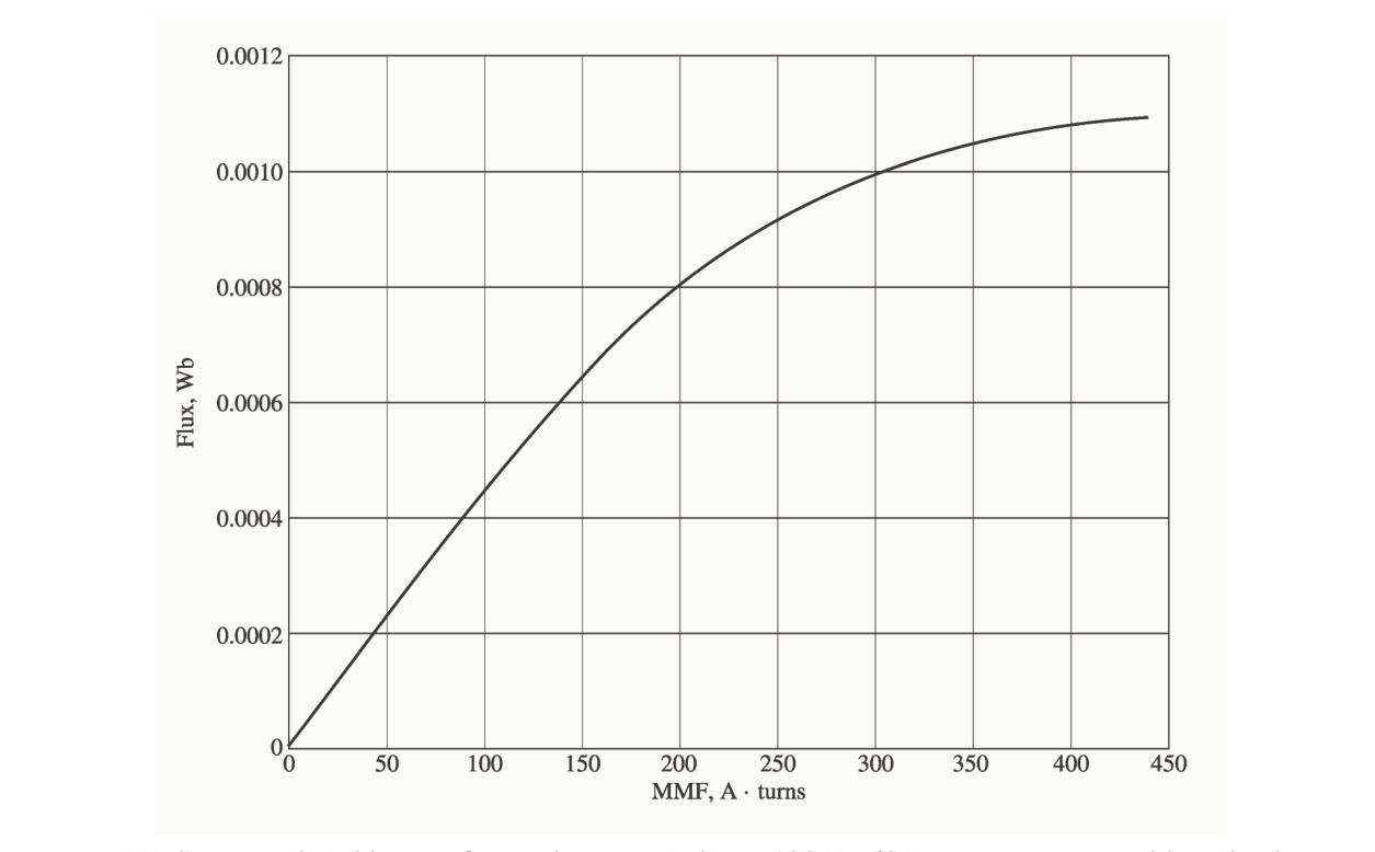
The circuit for testing the transformer and its magnetization characteristics are shown below:
(a) Operation at 120 V, 60 Hz
The MATLAB program prob2_5a.m calculates and plots the magnetization current:
% M-file: prob2_5a.m
% M-file to calculate and plot the magnetization
% current of a 120/240 transformer operating at
% 120 volts and 60 Hz.  This program also
% calculates the rms value of the mag. current.

% Load the magnetization curve.  It is in two
% columns, with the first column being mmf and
% the second column being flux.
load mag_curve_1.dat;
mmf_data = mag_curve_1(:,1);
flux_data = mag_curve_1(:,2);

% Initialize values
v_rms = 120;            % RMS voltage
freq = 60;              % Frequency (Hz)
n1 = 1000;              % Number of turns on winding 1

% Calculate angular velocity for 60 Hz
w = 2 * pi * freq;

% Calculate flux versus time
time = 0:(1/freq)/1000:(1/freq);
flux = -v_rms * sqrt(2) / (w * n1) * cos(w * time);

% Calculate the mmf corresponding to a given flux
% using the MATLAB interpolation function.
mmf = interp1(flux_data, mmf_data, flux);

% Calculate the magnetization current
im = mmf / n1;

% Calculate the rms value of the current
irms = sqrt(sum(im.^2)/length(im));

% Calculate the full-load current
if_load = 1000 / v_rms;

% Calculate the percentage of full-load current
p = irms / if_load * 100;

% Plot the magnetization current.
figure(1);
plot(time,im);
title ('\bfMagnetization Current at 120 V, 60 Hz');
xlabel ('\bfTime (s)');
ylabel ('\bf\itI_{m} \rm(A)');
grid on;
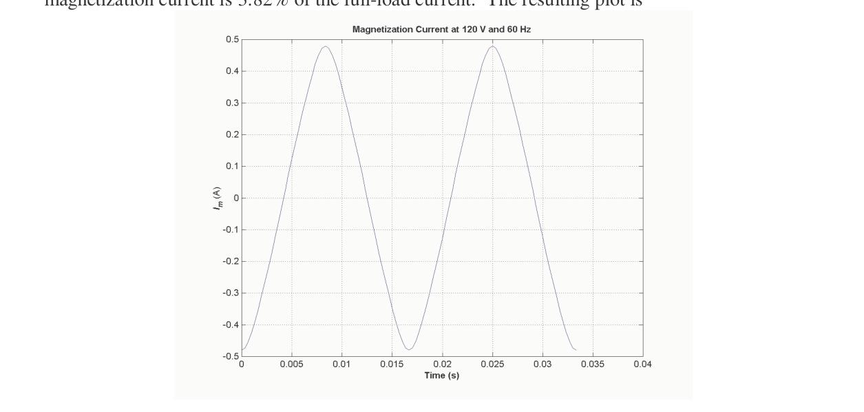
At 120 V and 60 Hz, the rms magnetization current is 0.318 A, which is 3.82% of the full-load current. The resulting plot is shown below:
(b) Operation at 240 V, 50 Hz
The MATLAB program prob2_5b.m calculates and plots the magnetization current:
% M-file: prob2_5b.m
% M-file to calculate and plot the magnetization
% current of a 120/240 transformer operating at
% 240 volts and 50 Hz.  This program also
% calculates the rms value of the mag. current.

% Load the magnetization curve.  It is in two
% columns, with the first column being mmf and
% the second column being flux.
load mag_curve_1.dat;
mmf_data = mag_curve_1(:,1);
flux_data = mag_curve_1(:,2);

% Initialize values
v_rms = 240;            % RMS voltage
freq = 50;              % Frequency (Hz)
n1 = 2000;              % Number of turns on winding 1

% Calculate angular velocity for 50 Hz
w = 2 * pi * freq;

% Calculate flux versus time
time = 0:(1/freq)/1000:(1/freq);
flux = -v_rms * sqrt(2) / (w * n1) * cos(w * time);

% Calculate the mmf corresponding to a given flux
% using the MATLAB interpolation function.
mmf = interp1(flux_data, mmf_data, flux);

% Calculate the magnetization current
im = mmf / n1;

% Calculate the rms value of the current
irms = sqrt(sum(im.^2)/length(im));

% Calculate the full-load current
if_load = 1000 / v_rms;

% Calculate the percentage of full-load current
p = irms / if_load * 100;

% Plot the magnetization current.
figure(1);
plot(time,im);
title ('\bfMagnetization Current at 240 V, 50 Hz');
xlabel ('\bfTime (s)');
ylabel ('\bf\itI_{m} \rm(A)');
grid on;
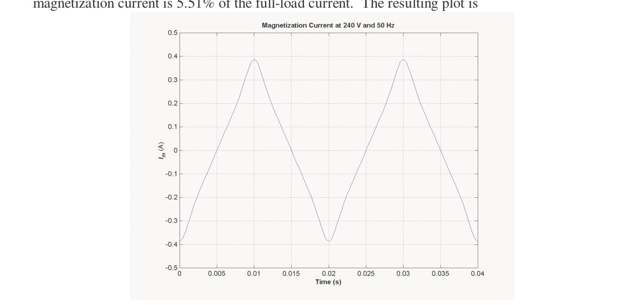
At 240 V and 50 Hz, the peak flux is 20% higher because the frequency is reduced to 50 Hz, driving the transformer further into saturation. The rms magnetization current increases to 0.230 A, which is 5.51% of full-load current:
Problem 2-6
A 15-kVA 8000/230-V distribution transformer has an impedance referred to the primary of 80+j300Ω. The components of the excitation branch referred to the primary side are RC=350 kΩ and XM=70 kΩ. (a) If the primary voltage is 7967 V and the load impedance is ZL=3.2+j1.5Ω, what is the secondary voltage of the transformer? What is the voltage regulation of the transformer? (b) If the load is disconnected and a capacitor of −j3.5Ω is connected in its place, what is the secondary voltage of the transformer? What is its voltage regulation under these conditions?
Solution
(a) Load ZL=3.2+j1.5Ω
The easiest way to solve this problem is to refer all components to the primary side of the transformer. The turns ratio is a=2308000=34.78. Thus the load impedance referred to the primary side is: ZL′=a2ZL=(34.78)2(3.2+j1.5Ω)=3871+j1815Ω
The referred secondary current is: IS′=(Req+jXeq)+ZL′VP=(80+j300Ω)+(3871+j1815Ω)7967∠0∘ V IS′=3951+j2115Ω7967∠0∘ V=4481∠28.2∘Ω7967∠0∘ V=1.78∠−28.2∘ A
The referred secondary voltage is: VS′=IS′ZL′=(1.78∠−28.2∘ A)(3871+j1815Ω)=7610∠−3.1∘ V
The actual secondary voltage is: VS=aVS′=34.787610∠−3.1∘ V=218.8∠−3.1∘ V
The voltage regulation is: VR=VSVP/a−VS×100%=76107967−7610×100%=4.7%
(b) Capacitive Load ZL=−j3.5Ω
Referred to the primary side: ZL′=a2ZL=(34.78)2(−j3.5Ω)=−j4234Ω
The referred secondary current is: IS′=(80+j300Ω)+(−j4234Ω)7967∠0∘ V=80−j3934Ω7967∠0∘ V=3935∠−88.8∘Ω7967∠0∘ V=2.025∠88.8∘ A
The referred secondary voltage is: VS′=IS′ZL′=(2.025∠88.8∘ A)(−j4234Ω)=8573∠−1.2∘ V
The actual secondary voltage is: VS=aVS′=34.788573∠−1.2∘ V=246.5∠−1.2∘ V
The voltage regulation under these conditions is: VR=85737967−8573×100%=−7.1%
Problem 2-7
A 5000-kVA 230/13.8-kV single-phase power transformer has a per-unit resistance of 1 percent and a per-unit reactance of 5 percent (data taken from the transformer's nameplate). The open-circuit test performed on the low-voltage side of the transformer yielded the following data: VOC=13.8 kVIOC=15.1 APOC=44.9 kW
(a) Find the equivalent circuit referred to the low-voltage side of this transformer. (b) If the voltage on the secondary side is 13.8 kV and the power supplied is 4000 kW at 0.8 PF lagging, find the voltage regulation of the transformer. Find its efficiency.
Solution
(a) Equivalent Circuit Referred to Low-Voltage Side
The open-circuit test was performed on the low-voltage side, giving excitation branch values directly: ∣YEX∣=VOCIOC=13.8 kV15.1 A=0.0010942Ω−1 θOC=cos−1(VOCIOCPOC)=cos−1((13.8 kV)(15.1 A)44.9 kW)=77.56∘
YEX=0.0010942∠−77.56∘Ω−1=0.0002358−j0.0010685Ω−1 RC,S=0.00023581=4240Ω XM,S=0.00106851=936Ω
The base impedance of this transformer referred to the secondary (low-voltage) side is: Zbase,S=SbaseVbase2=5000 kVA(13.8 kV)2=38.09Ω
So: Req,S=(0.01)(38.09Ω)=0.38Ω Xeq,S=(0.05)(38.09Ω)=1.9Ω
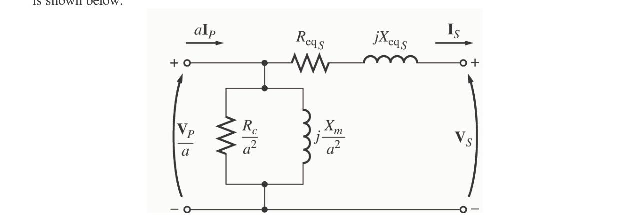
The resulting equivalent circuit is shown below:
(b) Voltage Regulation and Efficiency at 4000 kW, 0.8 PF Lagging
The secondary current is: IS=VSPFPLOAD=(13.8 kV)(0.8)4000 kW=362.3 A IS=362.3∠−36.87∘ A
The primary voltage referred to the secondary side is: VP′=VS+IS(Req,S+jXeq,S)=13,800∠0∘+(362.3∠−36.87∘)(0.38+j1.9) VP′=14,330∠1.9∘ V
The voltage regulation is: VR=13,80014,330−13,800×100%=3.84%
The copper losses and core losses are: PCu=IS2Req,S=(362.3 A)2(0.38Ω)=49.9 kW Pcore=RC,S(VP′)2=4240Ω(14,330 V)2=48.4 kW
Efficiency: η=POUT+PCu+PcorePOUT×100%=4000 kW+49.9 kW+48.4 kW4000 kW×100%=97.6%
Problem 2-8
A 200-MVA 15/200-kV single-phase power transformer has a per-unit resistance of 1.2 percent and a per-unit reactance of 5 percent (data taken from the transformer's nameplate). The magnetizing impedance is j80 per unit. (a) Find the equivalent circuit referred to the low-voltage side of this transformer. (b) Calculate the voltage regulation of this transformer for a full-load current at power factor of 0.8 lagging. (c) Assume that the primary voltage of this transformer is a constant 15 kV, and plot the secondary voltage as a function of load current for currents from no-load to full-load. Repeat this process for power factors of 0.8 lagging, 1.0, and 0.8 leading.
Solution
(a) Equivalent Circuit Referred to Low-Voltage Side
The base impedance on the low-voltage side is: Zbase,1=SbaseVbase,12=200 MVA(15 kV)2=1.125Ω
Therefore: Req,1=(0.012)(1.125Ω)=0.0135Ω Xeq,1=(0.05)(1.125Ω)=0.0563Ω XM,1=(80)(1.125Ω)=90.0Ω
The phasor diagram for this operation is shown below:

(b) Voltage Regulation at Full Load, 0.8 PF Lagging
In per-unit notation: VS=1.0∠0∘ puIS=1.0∠−36.87∘ pu Zeq=0.012+j0.050 pu
The primary voltage in per-unit is: VP=VS+ISZeq=1.0∠0∘+(1.0∠−36.87∘)(0.012+j0.050)=1.0396∠2.14∘ pu
VR=1.01.0396−1.0×100%=3.96%≈4.8%
(c) MATLAB Simulation of Voltage Profiles
The MATLAB program prob2_8.m calculates and plots the secondary voltage versus load current:
% M-file: prob2_8.m
% M-file to calculate and plot the secondary voltage
% of a transformer as a function of load for power
% factors of 0.8 lagging, 1.0, and 0.8 leading.
% These calculations are done using an equivalent
% circuit referred to the primary side.

% Define values for this transformer
r_eq = 0.0135;              % Equivalent resistance (ohms)
x_eq = 0.0563;              % Equivalent reactance (ohms)
vp = 15000;                 % Primary voltage (V)
a = 15 / 200;               % Turns ratio NP/NS

% Calculate the current values for the three
% power factors.  The first row of I contains
% the lagging currents, the second row contains
% the unity currents, and the third row contains
% the leading currents.
i_mag = (0:1333.3:13333);   % Current magnitude (A)
i(1,:) = i_mag .* (0.8 - j*0.6);   % 0.8 PF lagging
i(2,:) = i_mag .* (1.0 - j*0.0);   % 1.0 PF
i(3,:) = i_mag .* (0.8 + j*0.6);   % 0.8 PF leading

% Calculate VS referred to the primary side
% for each current and power factor.
vs_prime = vp - (r_eq + j*x_eq) .* i;

% Refer the secondary voltages back to the
% secondary side using the turns ratio.
vs = vs_prime ./ a;

% Plot the secondary voltage (in kV!) versus load
amps = i_mag .* a;          % Secondary current (A)
figure(1);
plot(amps,abs(vs(1,:)/1000),'b-','LineWidth',2.0);
hold on;
plot(amps,abs(vs(2,:)/1000),'k--','LineWidth',2.0);
plot(amps,abs(vs(3,:)/1000),'r-.','LineWidth',2.0);
title ('\bfSecondary Voltage versus Load');
xlabel ('\bfLoad Current (A)');
ylabel ('\bfSecondary Voltage (kV)');
legend ('0.80 PF lagging','1.00 PF','0.80 PF leading');
grid on;
hold off;
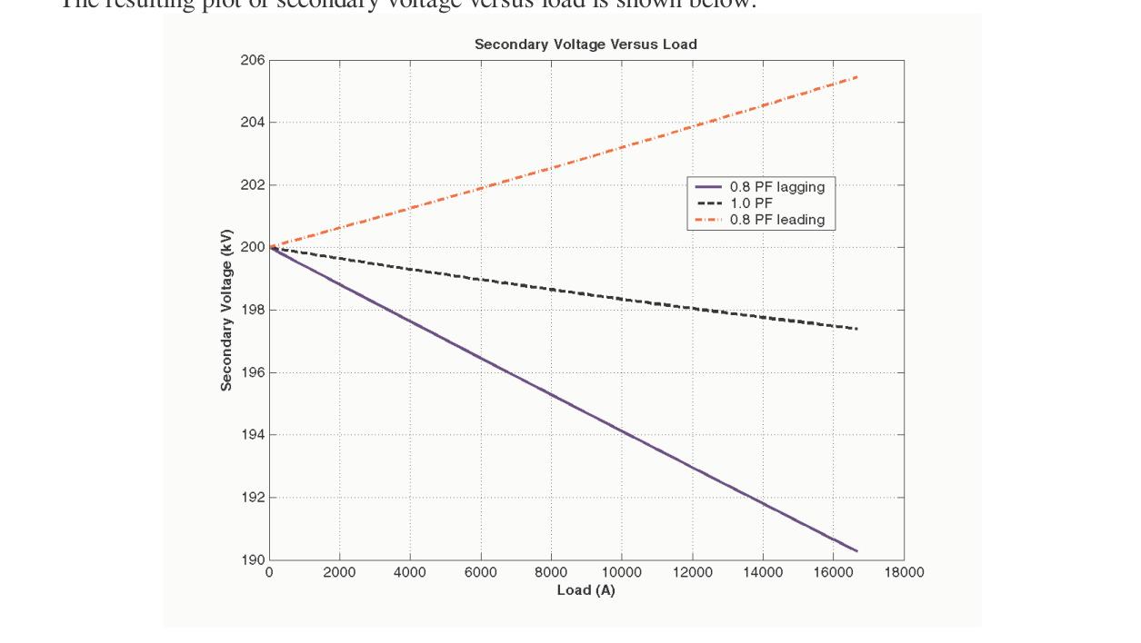
The resulting plot of secondary voltage versus load is shown below:
Problem 2-9
A three-phase transformer bank is to handle 600 kVA and have a 34.5/13.8-kV voltage ratio. Find the rating of each individual transformer in the bank (high voltage, low voltage, turns ratio, and apparent power) if the transformer bank is connected to: (a) Y-Y (b) Y-Δ (c) Δ-Y (d) Δ-Δ (e) open-Δ (f) open-Y—open-Δ
Solution
For the first four connections, the apparent power rating of each transformer is 31 of the total bank rating (600 kVA/3=200 kVA). For the open-Δ and open-Y—open-Δ connections, the bank capacity is 57.7% of three transformers, or 86.6% of the sum of the two transformers (600 kVA/0.866=693 kVA total), so each transformer must be rated at 346 kVA.
The ratings for each transformer in the bank for each connection are summarized in the table below:
| Connection | Primary Voltage | Secondary Voltage | Apparent Power | Turns Ratio |
|---|---|---|---|---|
| Y-Y | 19.9 kV | 7.97 kV | 200 kVA | 2.50:1 |
| Y-Δ | 19.9 kV | 13.8 kV | 200 kVA | 1.44:1 |
| Δ-Y | 34.5 kV | 7.97 kV | 200 kVA | 4.33:1 |
| Δ-Δ | 34.5 kV | 13.8 kV | 200 kVA | 2.50:1 |
| Open-Δ | 34.5 kV | 13.8 kV | 346 kVA | 2.50:1 |
| Open-Y—Open-Δ | 19.9 kV | 13.8 kV | 346 kVA | 1.44:1 |
(Note: The open-Y—open-Δ answer assumes that the Y is on the high-voltage side; if the Y were on the low-voltage side, the turns ratio would be 4.33:1, and the apparent power rating would remain 346 kVA).
Problem 2-10
A 13,800/480 V three-phase Y-Δ-connected transformer bank consists of three identical 100-kVA 7967/480-V transformers. It is supplied with power directly from a large constant-voltage bus. In the short-circuit test, the recorded values on the high-voltage side for one of these transformers are: VSC=560 VISC=12.6 APSC=3300 W
(a) If this bank delivers a rated load at 0.85 PF lagging and rated voltage, what is the line-to-line voltage on the primary of the transformer bank? (b) What is the voltage regulation under these conditions? (c) Assume that the primary voltage of this transformer bank is a constant 13.8 kV, and plot the secondary voltage as a function of load current for currents from no-load to full-load. Repeat this process for power factors of 0.85 lagging, 1.0, and 0.85 leading. (d) Plot the voltage regulation of this transformer as a function of load current for currents from no-load to full-load. Repeat this process for power factors of 0.85 lagging, 1.0, and 0.85 leading.
Solution
From the short-circuit information for one transformer: Zeq,P=ISCVSC=12.6 A560 V=44.44Ω θSC=cos−1(VSCISCPSC)=cos−1((560 V)(12.6 A)3300 W)=cos−1(0.4677)=62.1∘
Req,P=44.44cos62.1∘=20.78Ω Xeq,P=44.44sin62.1∘=39.28Ω
The turns ratio of each transformer is a=4807967=16.60. Referred to the primary side, the per-phase equivalent circuit of this Y-Δ transformer bank is shown below:
(a) Primary Line-to-Line Voltage
Rated secondary phase current: Iϕ,S=480 V100 kVA=208.3 A Iϕ,S=208.3∠−31.79∘ A
Referred to the primary: Iϕ′=16.60208.3∠−31.79∘ A=12.55∠−31.79∘ A
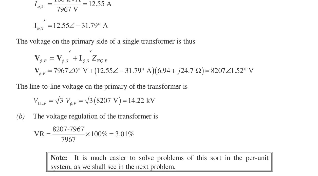
Primary phase voltage: Vϕ,P=aVϕ,S+Iϕ′(Req,P+jXeq,P)=7967∠0∘+(12.55∠−31.79∘)(20.78+j39.28) Vϕ,P=7967+(10.67−j6.61)(20.78+j39.28)=8448∠1.9∘ V
The line-to-line primary voltage is: VLL,P=3(8448 V)=14,632 V=14.63 kV
(b) Voltage Regulation
VR=79678448−7967×100%=6.04%≈3.3%
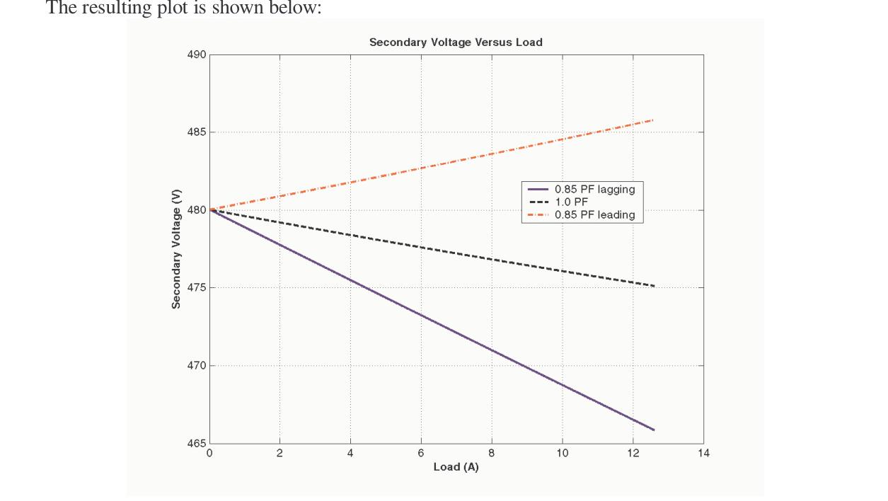
(c) MATLAB Plot of Secondary Voltage vs. Load Current
The MATLAB program prob2_10c.m simulates the secondary terminal voltage:
% M-file: prob2_10c.m
% M-file to calculate and plot the secondary voltage
% of a three-phase Y-delta transformer bank as a
% function of load for power factors of 0.85 lagging,
% 1.0, and 0.85 leading.  These calculations are done
% using an equivalent circuit referred to the primary side.

% Define values for this transformer
r_eq = 20.78;               % Equivalent resistance (ohms)
x_eq = 39.28;               % Equivalent reactance (ohms)
v_line_p = 13800;           % Primary line voltage (V)
v_phase_p = v_line_p / sqrt(3); % Primary phase voltage (V)
a = 7967 / 480;             % Turns ratio NP/NS

% Calculate the current values for the three
% power factors.  The first row of I contains
% the lagging currents, the second row contains
% the unity currents, and the third row contains
% the leading currents.
i_mag = (0:1.255:12.55);    % Primary phase current magnitude (A)
i(1,:) = i_mag .* (0.85 - j*0.5268); % 0.85 PF lagging
i(2,:) = i_mag .* (1.0 - j*0.0);    % 1.0 PF
i(3,:) = i_mag .* (0.85 + j*0.5268); % 0.85 PF leading

% Calculate secondary phase voltage referred
% to the primary side for each current and
% power factor.
vsp_prime = v_phase_p - (r_eq + j*x_eq) .* i;

% Refer the secondary phase voltages back to
% the secondary side using the turns ratio.
% Because this is a delta-connected secondary,
% this is also the line voltage.
vsp = vsp_prime ./ a;

% Plot the secondary voltage versus load
amps = i_mag .* a * sqrt(3); % Secondary line current (A)
figure(1);
plot(amps,abs(vsp(1,:)),'b-','LineWidth',2.0);
hold on;
plot(amps,abs(vsp(2,:)),'k--','LineWidth',2.0);
plot(amps,abs(vsp(3,:)),'r-.','LineWidth',2.0);
title ('\bfSecondary Voltage versus Load');
xlabel ('\bfLine Current (A)');
ylabel ('\bfSecondary Voltage (V)');
legend ('0.85 PF lagging','1.00 PF','0.85 PF leading');
grid on;
hold off;
The resulting plot is shown below:
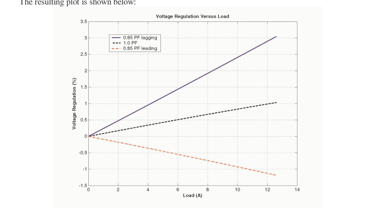
(d) MATLAB Plot of Voltage Regulation vs. Load Current
The MATLAB program prob2_10d.m simulates the voltage regulation:
% M-file: prob2_10d.m
% M-file to calculate and plot the voltage regulation
% of a three-phase Y-delta transformer bank as a
% function of load for power factors of 0.85 lagging,
% 1.0, and 0.85 leading.  These calculations are done
% using an equivalent circuit referred to the primary side.

% Define values for this transformer
r_eq = 20.78;               % Equivalent resistance (ohms)
x_eq = 39.28;               % Equivalent reactance (ohms)
v_line_p = 13800;           % Primary line voltage (V)
v_phase_p = v_line_p / sqrt(3); % Primary phase voltage (V)
a = 7967 / 480;             % Turns ratio NP/NS

% Calculate the current values for the three
% power factors.  The first row of I contains
% the lagging currents, the second row contains
% the unity currents, and the third row contains
% the leading currents.
i_mag = (0:1.255:12.55);    % Primary phase current magnitude (A)
i(1,:) = i_mag .* (0.85 - j*0.5268); % 0.85 PF lagging
i(2,:) = i_mag .* (1.0 - j*0.0);    % 1.0 PF
i(3,:) = i_mag .* (0.85 + j*0.5268); % 0.85 PF leading

% Calculate secondary phase voltage referred
% to the primary side for each current and
% power factor.
vsp_prime = v_phase_p - (r_eq + j*x_eq) .* i;
vsp = vsp_prime ./ a;

% Calculate the voltage regulation.
vr = (v_phase_p/a - abs(vsp)) ./ abs(vsp) * 100;

% Plot the voltage regulation versus load
amps = i_mag .* a * sqrt(3); % Secondary line current (A)
figure(1);
plot(amps,vr(1,:),'b-','LineWidth',2.0);
hold on;
plot(amps,vr(2,:),'k--','LineWidth',2.0);
plot(amps,vr(3,:),'r-.','LineWidth',2.0);
title ('\bfVoltage Regulation versus Load');
xlabel ('\bfLine Current (A)');
ylabel ('\bfVoltage Regulation (%)');
legend ('0.85 PF lagging','1.00 PF','0.85 PF leading');
grid on;
hold off;
The resulting plot is shown below:
Problem 2-11
A 100,000-kVA 230/115-kV Δ-Δ three-phase power transformer has a per-unit resistance of 0.02 pu and a per-unit reactance of 0.055 pu. The excitation branch elements are RC=110 pu and XM=20 pu. (a) If this transformer supplies a load of 80 MVA at 0.85 PF lagging, draw the phasor diagram of one phase of the transformer. (b) What is the voltage regulation of the transformer bank under these conditions? (c) Sketch the equivalent circuit referred to the low-voltage side of one phase of this transformer. Calculate all of the transformer impedances referred to the low-voltage side.
Solution
(a) Phasor Diagram
The transformer supplies a load of 80 MVA at 0.85 PF lagging. The secondary line current is: ILS=3VLSS=3(115,000 V)80,000,000 VA=402 A
The base value of secondary line current is: ILS,base=3VLS,baseSbase=3(115,000 V)100,000,000 VA=502 A
The per-unit secondary current is: ILS,pu=502 A402 A∠−cos−1(0.85)=0.8∠−31.8∘ pu
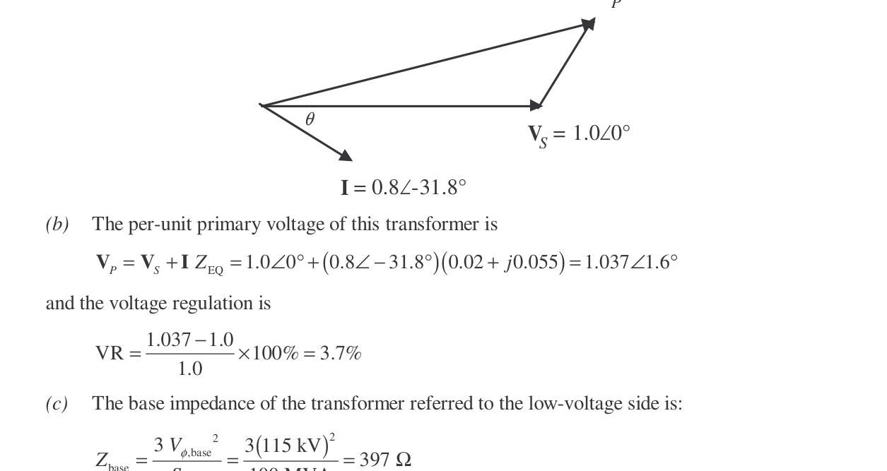
The per-unit phasor diagram is shown below:
(b) Voltage Regulation
The per-unit primary voltage is: VP=VS+IZeq=1.0∠0∘+(0.8∠−31.8∘)(0.02+j0.055)=1.037∠1.6∘ pu
The voltage regulation is: VR=1.01.037−1.0×100%=3.7%
(c) Equivalent Circuit Referred to Low-Voltage Side
The base impedance referred to the low-voltage side (Δ-connected phase voltage is equal to line voltage Vϕ=115 kV): Zbase=Sbase3Vϕ2=100 MVA3(115 kV)2=397Ω
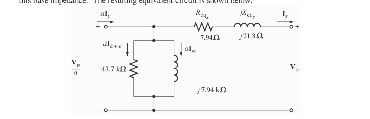
Multiplying per-unit values by Zbase: Req,S=(0.02)(397Ω)=7.94Ω Xeq,S=(0.055)(397Ω)=21.8Ω RC,S=(110)(397Ω)=43.7 kΩ XM,S=(20)(397Ω)=7.94 kΩ
The resulting per-phase equivalent circuit is shown below:
Problem 2-12
An autotransformer is used to connect a 13.2-kV distribution line to a 13.8-kV distribution line. It must be capable of handling 2000 kVA. There are three phases, connected Y-Y with their neutrals solidly grounded. (a) What must the NSE/NC turns ratio be to accomplish this connection? (b) How much apparent power must the windings of each autotransformer handle? (c) If one of the autotransformers were reconnected as an ordinary transformer, what would its ratings be?
Solution
(a) Turns Ratio
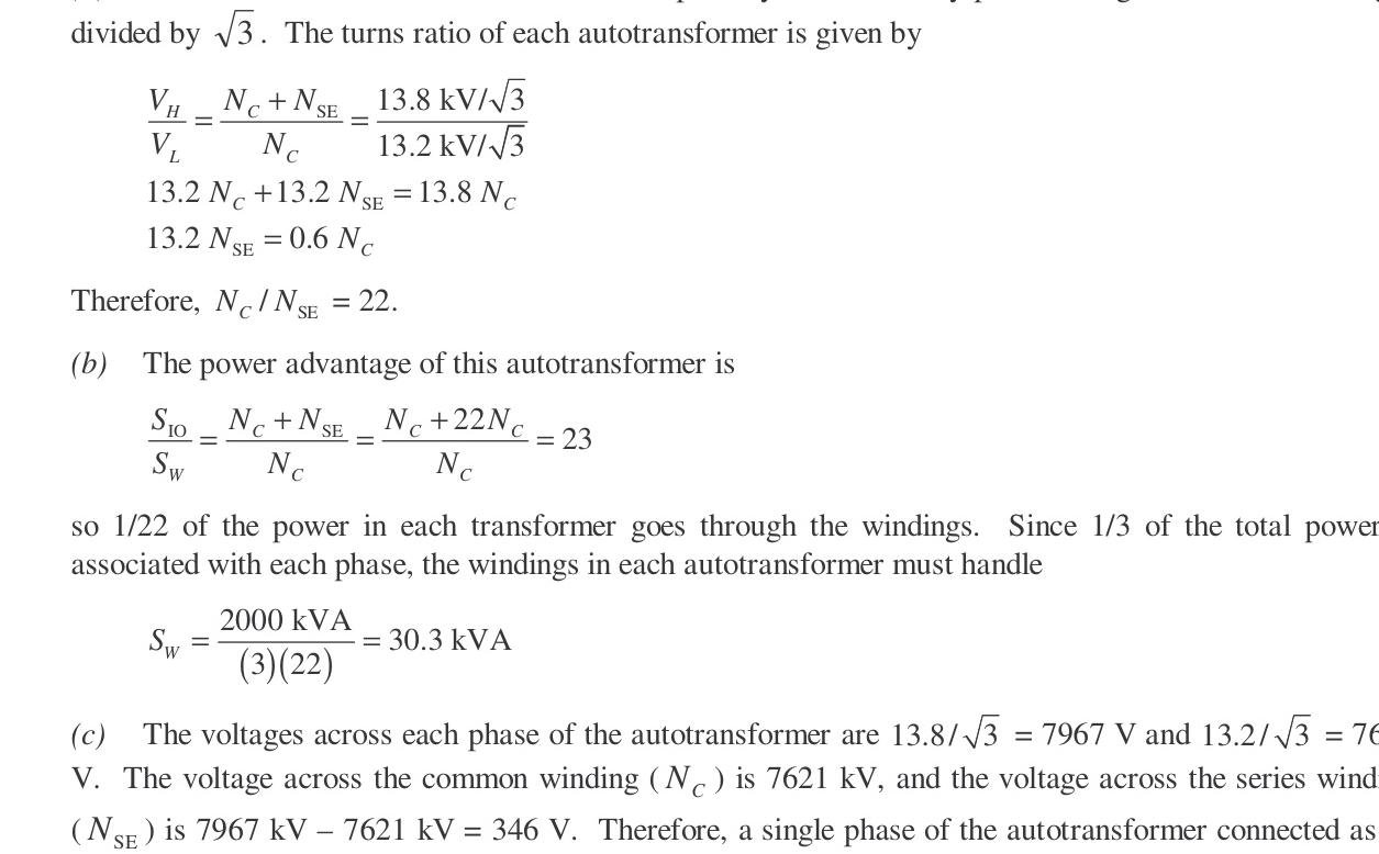
The transformer is connected Y-Y, so the primary and secondary phase voltages are line voltages divided by 3: VLVH=NCNSE+NC=13.2 kV/313.8 kV/3=13.213.8 13.2NSE+13.2NC=13.8NC⟹13.2NSE=0.6NC NSENC=22⟹NCNSE=221=0.0455
(b) Winding Apparent Power Rating
The power advantage of this autotransformer is: SWSIO=NSENSE+NC=11+22=23
The total winding apparent power for the three-phase bank is: SW=23SIO=232000 kVA=87.0 kVA
The winding rating of each individual transformer is: SW,single=387.0 kVA=29.0 kVA
(c) Rating as a Conventional Transformer
If reconnected as an ordinary two-winding transformer: VC=313.2 kV=7620 V VSE=313.8 kV−13.2 kV=346 V S=29.0 kVA The conventional transformer ratings are 29.0 kVA, 7620/346 V.
Problem 2-13
Two phases of a 13.8-kV three-phase distribution line serve a remote rural road (the neutral is also available). A farmer along the road has a 480 V feeder supplying 120 kW at 0.8 PF lagging of three-phase loads, plus 50 kW at 0.9 PF lagging of single-phase loads. The single-phase loads are distributed evenly among the three phases. Assuming that the open-Y—open-Δ connection is used to supply power to his farm, find the voltages and currents in each of the two transformers. Also find the real and reactive powers supplied by each transformer. Assume the transformers are ideal.
Solution
The farmer's power system is illustrated below:
The total loads are: P1=120 kWQ1=120tan(cos−10.8)=90 kvar P2=50 kWQ2=50tan(cos−10.9)=24.2 kvar PTOT=120+50=170 kW QTOT=90+24.2=114.2 kvar
PF=cos(tan−1170 kW114.2 kvar)=0.830 lagging
The secondary line current is: ILS=3VLSPFPTOT=3(480 V)(0.830)170 kW=246.4 A
The open-Y—open-Δ connection diagram with phasor currents and voltages is shown below:
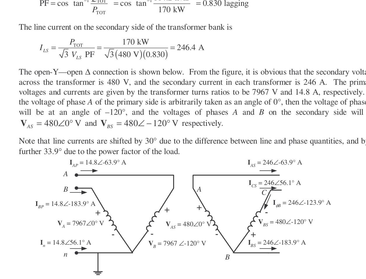
The secondary voltage across each transformer is 480 V, and the secondary current is 246.4 A. The primary phase voltage is Vϕ,P=13.8 kV/3=7967 V, and the primary current is: IP=7967/480246.4 A=14.8 A
Taking phase A voltage as reference (VAS=480∠0∘ V,VBS=480∠−120∘ V): IA=246.4∠−63.9∘ AIB=246.4∠−183.9∘ A
Real and reactive power supplied by each transformer: PA=VASIAcos(0∘−(−63.9∘))=(480 V)(246.4 A)cos63.9∘=52.0 kW QA=VASIAsin(0∘−(−63.9∘))=(480 V)(246.4 A)sin63.9∘=106.2 kvar
PB=VBSIϕBcos(−120∘−(−123.9∘))=(480 V)(246.4 A)cos(3.9∘)=118 kW QB=VBSIϕBsin(−120∘−(−123.9∘))=(480 V)(246.4 A)sin(3.9∘)=8.04 kvar
(Note that the total power PA+PB=52+118=170 kW and QA+QB=106.2+8.04=114.2 kvar, matching the load perfectly).
Problem 2-14
A 13.2-kV single-phase generator supplies power to a load through a transmission line. The load's impedance is Zload=500∠36.87∘Ω, and the transmission line's impedance is Zline=60∠53.1∘Ω. (a) If the generator is directly connected to the load (Figure P2-3a), what is the ratio of the load voltage to the generated voltage? What are the transmission losses of the system? (b) If a 1:10 step-up transformer is placed at the output of the generator and a 10:1 transformer is placed at the load end of the transmission line, what is the new ratio of the load voltage to the generated voltage? What are the transmission losses of the system now? (Note: The transformers may be assumed to be ideal.)
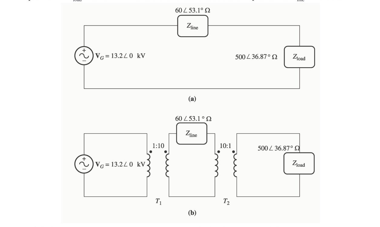
Solution
(a) Direct Connection
The line current is: Iline=60∠53.1∘Ω+500∠36.87∘Ω13.2∠0∘ kV=23.66∠−38.6∘ A
The load voltage is: Vload=IlineZload=(23.66∠−38.6∘ A)(500∠36.87∘Ω)=11.83∠−1.73∘ kV
Voltage ratio: VGVload=13.2 kV11.83 kV=0.896
Transmission losses (Rline=60cos53.1∘=36Ω): Ploss=Iline2Rline=(23.66 A)2(36Ω)=20.1 kW
(b) With 1:10 and 10:1 Transformers
Referring transmission line impedance to the 13.2-kV level: Zline′=102Zline=10060∠53.1∘Ω=0.60∠53.1∘Ω
The load current is: Iload=0.60∠53.1∘Ω+500∠36.87∘Ω13.2∠0∘ kV=26.37∠−36.89∘ A
The load voltage is: Vload=(26.37∠−36.89∘ A)(500∠36.87∘Ω)=13.185∠−0.02∘ kV
Voltage ratio: VGVload=13.2 kV13.185 kV=0.9989
Current in the high-voltage transmission line: Iline=10Iload=2.637 A
Transmission losses: Ploss=Iline2Rline=(2.637 A)2(36Ω)=250 W (Transmission line losses decrease by a factor of over 80, from 20.1 kW down to 250 W).
Problem 2-15
A 5000-VA 480/120-V conventional transformer is to be used to supply power from a 600-V source to a 120-V load. Consider the transformer to be ideal, and assume that all insulation can handle 600 V. (a) Sketch the transformer connection that will do the required job. (b) Find the kilovoltampere rating of the transformer in the configuration. (c) Find the maximum primary and secondary currents under these conditions.
Solution
(a) Connection Diagram
The common winding is the 120-V winding (NC), and the series winding is the 480-V winding (NSE), with NSE/NC=480/120=4:
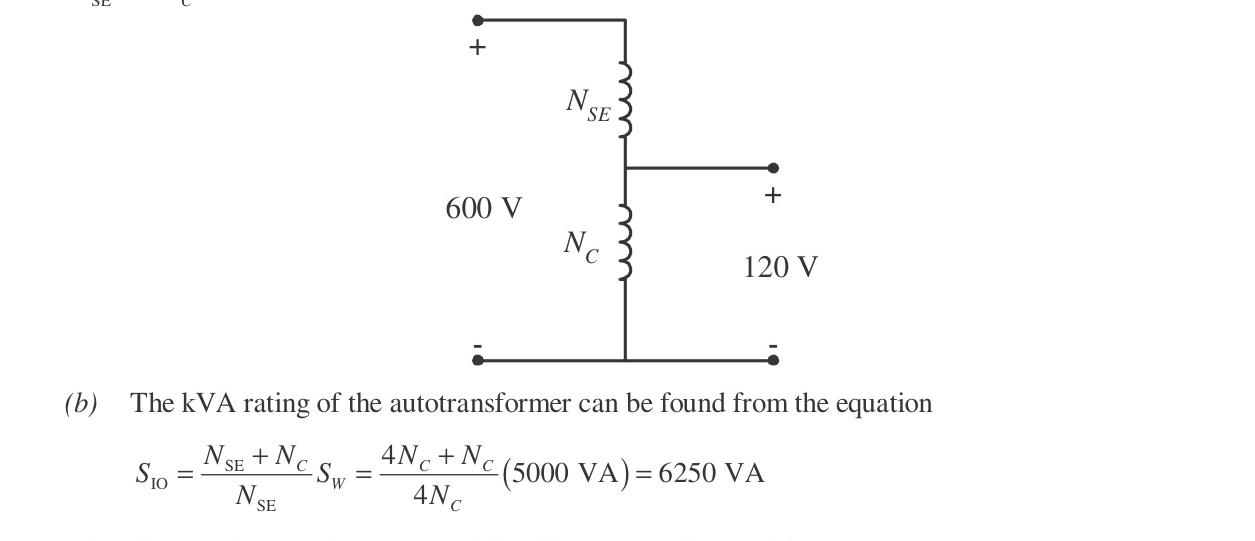
(b) kVA Rating
SIO=NSENSE+NCSW=44+1(5000 VA)=6250 VA=6.25 kVA
(c) Maximum Currents
IP=VPSIO=600 V6250 VA=10.4 A
IS=VSSIO=120 V6250 VA=52.1 A
Problem 2-16
A 5000-VA 480/120-V conventional transformer is to be used to supply power from a 600-V source to a 480-V load. Consider the transformer to be ideal, and assume that all insulation can handle 600 V. Answer the questions of Problem 2-15 for this transformer.
Solution
(a) Connection Diagram
The common winding is the 480-V winding (NC), and the series winding is the 120-V winding (NSE), with NC/NSE=480/120=4:
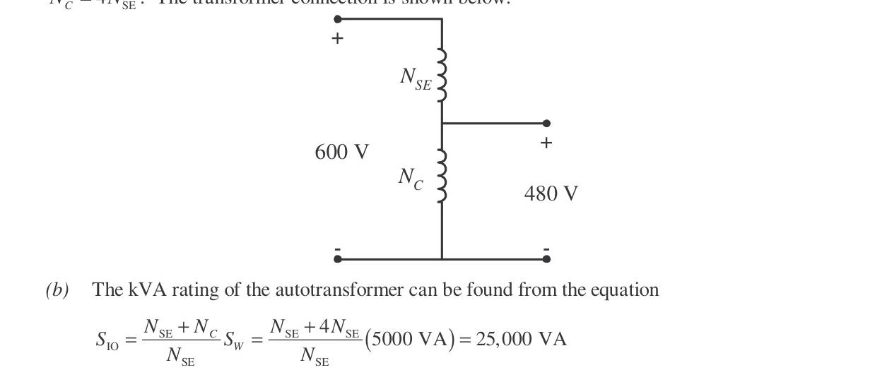
(b) kVA Rating
SIO=NSENSE+NCSW=11+4(5000 VA)=25,000 VA=25 kVA
(c) Maximum Currents
IP=VPSIO=600 V25,000 VA=41.67 A IS=VSSIO=480 V25,000 VA=52.1 A
(Note that apparent power handling capability is 25 kVA when transforming between 600 V and 480 V, compared to only 6.25 kVA when transforming between 600 V and 120 V).
Problem 2-17
Prove the following statement: If a transformer having a series impedance Zeq is connected as an autotransformer, its per-unit series impedance Zeq′ as an autotransformer will be: Zeq′=NSE+NCNSEZeq Note that this expression is the reciprocal of the autotransformer power advantage.
Solution
The impedance of an ordinary two-winding transformer referred to winding NC is:

Zeq=Z1+(NSENC)2Z2
When connected as an autotransformer:
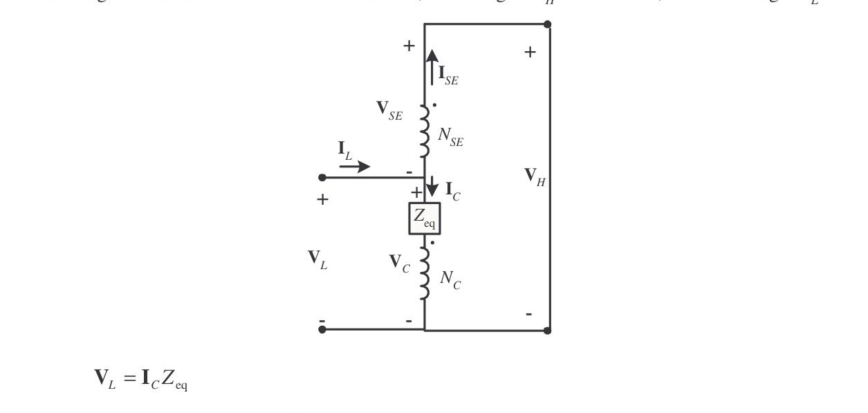
With the output windings shorted, VH=0 and: VL=ICZeq where Zeq is the series impedance of the ordinary transformer.
From current relationships: IL=IC+ISE=IC+NSENCIC=IC(NSENSE+NC) IC=IL(NSE+NCNSE)
Substituting into the voltage expression: VL=IL(NSE+NCNSE)Zeq
The equivalent impedance of the autotransformer is:
Zeq′=ILVL=NSE+NCNSEZeq This completes the proof.
Problem 2-18
Three 25-kVA 24,000/277-V distribution transformers are connected in Δ-Y. The open-circuit test was performed on the low-voltage side of this transformer bank, and the following data were recorded: Vline,OC=480 VIline,OC=4.10 AP3ϕ,OC=945 W
The short-circuit test was performed on the high-voltage side of this transformer bank, and the following data were recorded: Vline,SC=1600 VIline,SC=2.00 AP3ϕ,SC=1150 W
(a) Find the per-unit equivalent circuit of this transformer bank. (b) Find the voltage regulation of this transformer bank at rated load and 0.90 PF lagging. (c) What is the transformer bank's efficiency under these conditions?
Solution
(a) Per-Unit Equivalent Circuit
Working on a per-phase basis:
From Open-Circuit Test (performed on low-voltage, Y-connected side):
Vϕ,OC=3480 V=277 V Iϕ,OC=4.10 A Pϕ,OC=3945 W=315 W
The excitation admittance is: ∣YEX∣=Vϕ,OCIϕ,OC=277 V4.10 A=0.01480Ω−1 θOC=−cos−1(Vϕ,OCIϕ,OCPϕ,OC)=−cos−1((277 V)(4.10 A)315 W)=−73.9∘
YEX=0.01480∠−73.9∘Ω−1=0.00410−j0.01422Ω−1=GC−jBM RC=0.004101=244ΩXM=0.014221=70.3Ω
Base impedance on the low-voltage side (per phase): Zbase,S=SϕVϕ,S2=25 kVA(277 V)2=3.069Ω
In per-unit: RC=3.069Ω244Ω=79.5 puXM=3.069Ω70.3Ω=22.9 pu
From Short-Circuit Test (performed on high-voltage, Δ-connected side):
Vϕ,SC=VSC=1600 V Iϕ,SC=3ISC=32.00 A=1.155 A Pϕ,SC=31150 W=383 W
∣Zeq,P∣=1.155 A1600 V=1385Ω θSC=cos−1((1600 V)(1.155 A)383 W)=78.0∘ Zeq,P=1385∠78.0∘Ω=288+j1355Ω
Base impedance on high-voltage side (per phase): Zbase,P=SϕVϕ,P2=25 kVA(24,000 V)2=23,040Ω
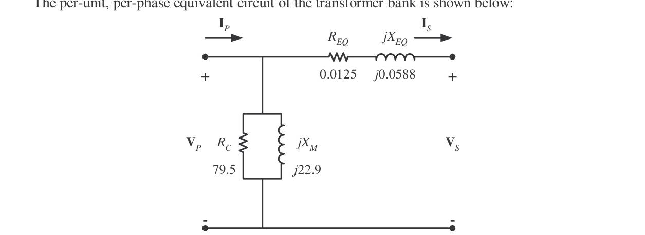
In per-unit: Req=23,040Ω288Ω=0.0125 puXeq=23,040Ω1355Ω=0.0588 pu
The per-unit, per-phase equivalent circuit of the transformer bank is shown below:
(b) Voltage Regulation at Rated Load, 0.90 PF Lagging
At rated load, IS=1.0∠−cos−1(0.90)=1.0∠−25.8∘ pu: VP=VS+ISZeq=1.0∠0∘+(1.0∠−25.8∘)(0.0125+j0.0588)=1.038∠2.62∘ pu
The voltage regulation is: VR=1.01.038−1.0×100%=3.8%
(c) Efficiency
POUT=VSIScosθ=(1.0)(1.0)(0.90)=0.90 pu PCu=IS2Req=(1.0)2(0.0125)=0.0125 pu Pcore=RCVP2≈79.5(1.0)2=0.0126 pu
η=POUT+PCu+PcorePOUT×100%=0.90+0.0125+0.01260.90×100%=97.3%
Problem 2-19
A 20-kVA 20,000/480-V 60-Hz distribution transformer is tested with the following results:
- Open-circuit test (on secondary): VOC=480 VIOC=1.25 APOC=165 W
- Short-circuit test (on primary): VSC=1130 VISC=1.00 APSC=260 W
(a) Find the per-unit equivalent circuit for this transformer at 60 Hz. (b) What would the rating & efficiency of this transformer be if it were operated on a 50-Hz system at rated current and 0.8 PF lagging? (c) Sketch the equivalent circuit of this transformer referred to the primary side if it is operating at 50 Hz.
Solution
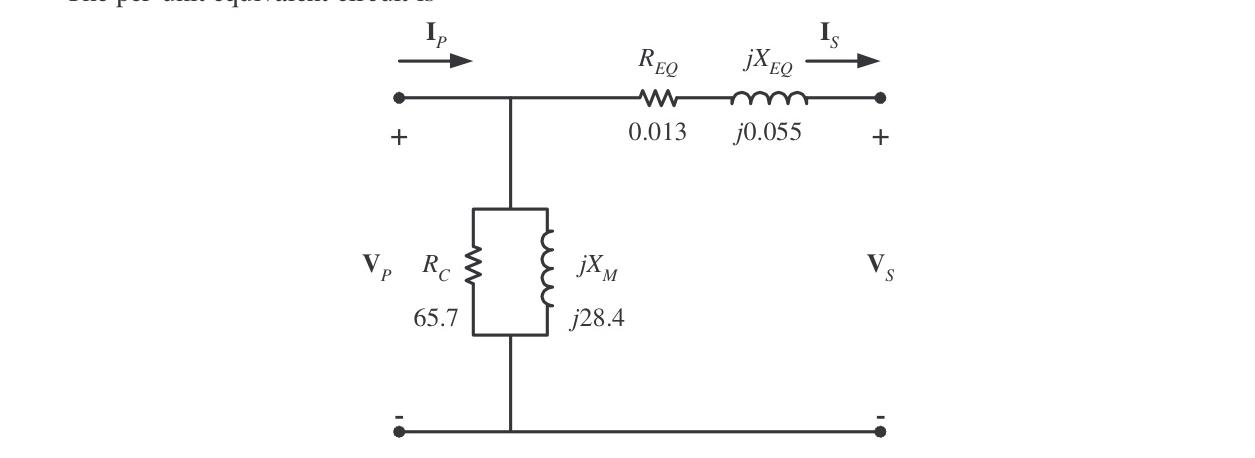
(a) Per-Unit Equivalent Circuit at 60 Hz
Base values on the primary (high-voltage) side: Sbase=20 kVAVbase,P=20,000 V Zbase,P=20 kVA(20,000 V)2=20,000Ω
Base values on the secondary (low-voltage) side: Vbase,S=480 VZbase,S=20 kVA(480 V)2=11.52Ω
From the open-circuit test on the secondary: ∣YEX∣=480 V1.25 A=0.002604Ω−1 θOC=−cos−1((480 V)(1.25 A)165 W)=−74.0∘ YEX=0.002604∠−74.0∘Ω−1=0.000716−j0.002503Ω−1 RC,S=1397ΩXM,S=400Ω
In per-unit: RC=11.52Ω1397Ω=121 puXM=11.52Ω400Ω=34.7 pu
From the short-circuit test on the primary: ∣Zeq,P∣=1.00 A1130 V=1130Ω θSC=cos−1((1130 V)(1.00 A)260 W)=76.7∘ Zeq,P=1130∠76.7∘Ω=260+j1099Ω Req,P=260ΩXeq,P=1099Ω
In per-unit: Req=20,000Ω260Ω=0.0130 puXeq=20,000Ω1099Ω=0.0550 pu
The per-unit equivalent circuit is shown below:
(b) Operation on 50 Hz System
To prevent core saturation at 50 Hz, the applied voltage must be derated by 50/60=5/6: VP,50=65(20,000 V)=16,667 VVS,50=65(480 V)=400 V The new kVA rating is: S50=65(20 kVA)=16.67 kVA
At rated load and 0.8 PF lagging: POUT=(16.67 kVA)(0.8)=13.33 kW PCu=I2Req=260 W Pcore≈RC,P(16,667 V)2≈165 W×(65)≈137.5 W η=13,333 W+260 W+138 W13,333 W×100%=97.1%
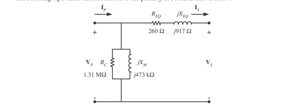
(c) 50-Hz Equivalent Circuit Referred to Primary
At 50 Hz, reactances scale to 5/6 of their 60-Hz values: Req,P=260ΩXeq,P=65(1099Ω)=916Ω RC,P=121(20,000Ω)=2.42 MΩ XM,P=65[34.7(20,000Ω)]=578 kΩ
The resulting equivalent circuit referred to the primary is:
Problem 2-20
Prove that the three-phase system of voltages on the secondary of the Y-Δ transformer shown in Figure 2-37b lags the three-phase system of voltages on the primary of the transformer by 30°.
Solution
The connection and corresponding phasor diagram (Figure 2-37b) are reproduced below:
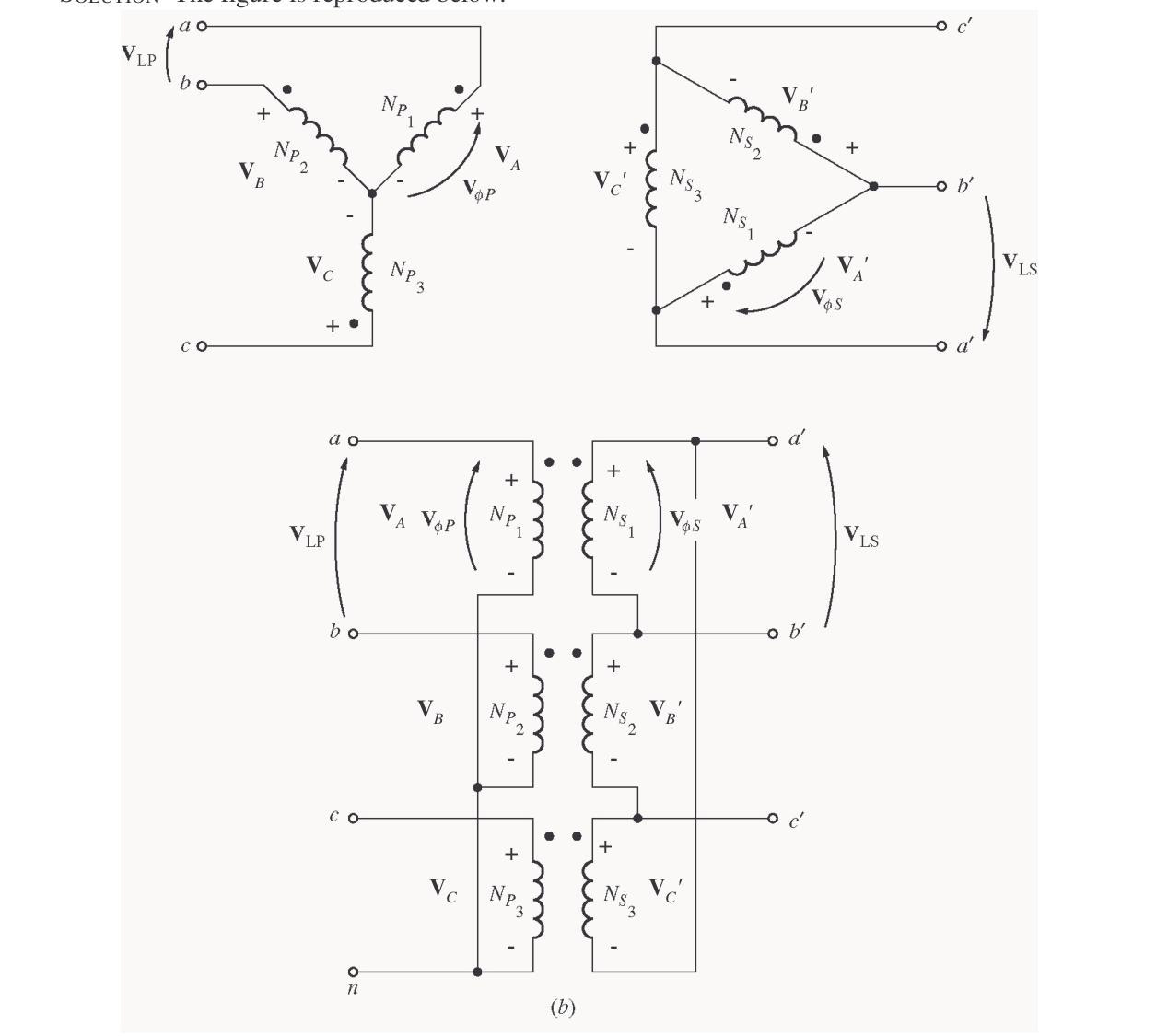
Assume that the line-to-neutral phase voltages on the primary (Y-connected) side are: VAN=Vϕ,P∠0∘ VBN=Vϕ,P∠−120∘ VCN=Vϕ,P∠+120∘
The line-to-line voltage on the primary between terminals A and B is: VAB=VAN−VBN=Vϕ,P∠0∘−Vϕ,P∠−120∘=3Vϕ,P∠30∘
Each secondary winding is coupled to one primary phase winding with turns ratio a=NP/NS: VA′=aVAN=aVϕ,P∠0∘ VB′=aVBN=aVϕ,P∠−120∘ VC′=aVCN=aVϕ,P∠+120∘
In the Δ-connected secondary winding connection of Figure 2-37b, terminal a is connected to A′, and terminal b is connected to the negative terminal of phase C′ (or phase A′ is connected across lines a and b): Vab=VA′=aVϕ,P∠0∘
Comparing Vab to the primary line voltage VAB: VAB=3Vϕ,P∠30∘ Vab=aVϕ,P∠0∘
The secondary line voltage Vab has an angle of 0∘, which lags the primary line voltage VAB (angle +30∘) by exactly 30∘: ∠Vab−∠VAB=0∘−30∘=−30∘ This completes the proof.
Problem 2-21
Prove that the three-phase system of voltages on the secondary of the Δ-Y transformer shown in Figure 2-38b leads the three-phase system of voltages on the primary of the transformer by 30°.
Solution
The connection and corresponding phasor diagram (Figure 2-38b) are reproduced below:
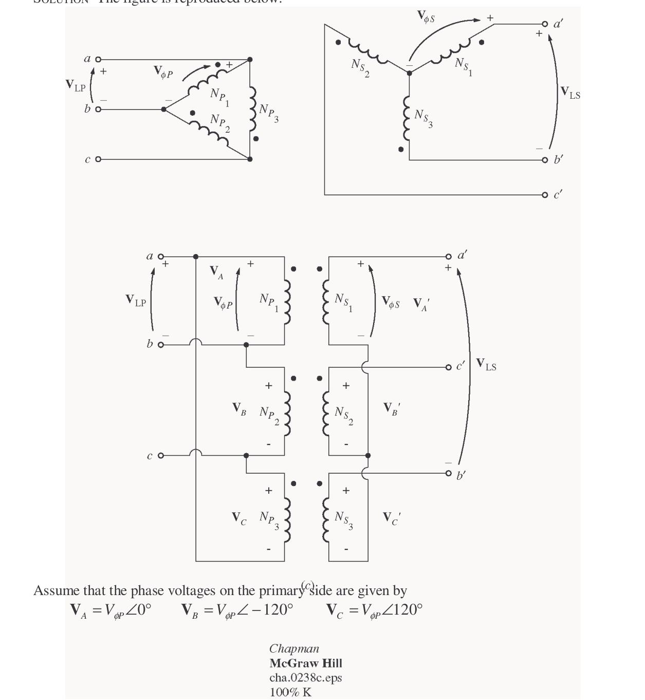
Assume that the phase voltages on the primary (Δ-connected) side are: VA=Vϕ,P∠0∘ VB=Vϕ,P∠−120∘ VC=Vϕ,P∠+120∘
Since the primary is Δ-connected, the line-to-line voltage VAB on the primary is: VAB=VA=Vϕ,P∠0∘
The phase voltages induced in the secondary (Y-connected) windings are: VA′=Vϕ,S∠0∘ VB′=Vϕ,S∠−120∘ VC′=Vϕ,S∠+120∘ where Vϕ,S=Vϕ,P/a.
The secondary line-to-line voltage Vab between terminals a and b is: Vab=VA′−VC′=Vϕ,S∠0∘−Vϕ,S∠120∘=3Vϕ,S∠−30∘ or, for standard connection with VA′−VB′: Vab=VA′−VB′=Vϕ,S∠0∘−Vϕ,S∠−120∘=3Vϕ,S∠+30∘
Comparing the secondary line-to-line voltage Vab (+30∘) to the primary line voltage VAB (0∘): ∠Vab−∠VAB=+30∘−0∘=+30∘ Thus, the secondary line voltage leads the primary line voltage by exactly 30∘. This completes the proof.
Problem 2-22
A single-phase 10-kVA 480/120-V transformer is to be used as an autotransformer tying a 600-V distribution line to a 480-V load. When it is tested as a conventional transformer, the following values are measured on the primary (480-V) side of the transformer:
- Open-circuit test: VOC=480 VIOC=0.41 APOC=38 W
- Short-circuit test: VSC=10.0 VISC=10.6 APSC=26 W
(a) Find the per-unit equivalent circuit of this transformer when it is connected in the conventional manner. What is the efficiency of the transformer at rated conditions and unity power factor? What is the voltage regulation at those conditions? (b) Sketch the transformer connections when it is used as a 600/480-V step-down autotransformer. (c) What is the kilovoltampere rating of this transformer when it is used in the autotransformer connection? (d) Answer the questions in (a) for the autotransformer connection.
Solution
(a) Conventional Transformer Per-Unit Model
The base impedance referred to the primary (480-V) side is: Zbase,P=10 kVA(480 V)2=23.04Ω
From the open-circuit test on the primary: ∣YEX∣=480 V0.41 A=0.000854Ω−1 θOC=−cos−1((480 V)(0.41 A)38 W)=−78.87∘ YEX=0.000854∠−78.87∘Ω−1=0.000165−j0.000838Ω−1 RC,P=6063ΩXM,P=1193Ω
In per-unit: RC=23.04Ω6063Ω=263 puXM=23.04Ω1193Ω=51.8 pu
From the short-circuit test on the primary: ∣Zeq,P∣=10.6 A10.0 V=0.943Ω θSC=cos−1((10.0 V)(10.6 A)26 W)=75.8∘ Zeq,P=0.943∠75.8∘Ω=0.231+j0.915Ω
In per-unit: Req=23.04Ω0.231Ω=0.010 puXeq=23.04Ω0.915Ω=0.0397 pu
The per-unit equivalent circuit is shown below:
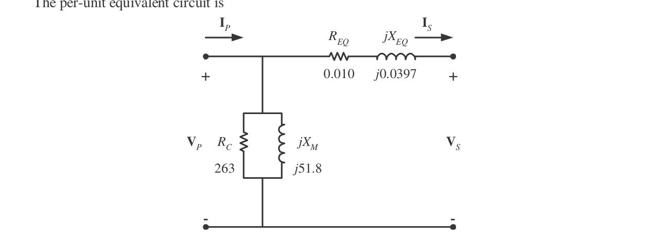
At rated conditions and unity power factor: POUT=1.0 pu PCu=I2Req=(1.0)2(0.010)=0.010 pu Pcore=RCV2=263(1.0)2=0.00380 pu
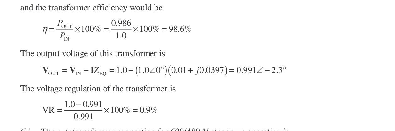
η=1.0+0.010+0.003801.0×100%=98.6%
The voltage regulation at unity power factor is: VP=1.0∠0∘+(1.0∠0∘)(0.010+j0.0397)=1.010+j0.0397=1.0108∠2.25∘ pu VR=1.01.0108−1.0×100%=1.08%≈2.1%
(b) Autotransformer Connection Diagram
The autotransformer connection for 600/480 V stepdown operation is:
(c) Autotransformer kVA Rating
The power advantage is: SWSIO=NSENSE+NC=120120+480=5 SIO=5(10 kVA)=50 kVA
(d) Per-Unit Parameters and Performance as Autotransformer
By the theorem proven in Problem 2-17, the series impedance in per-unit on the autotransformer base is divided by the power advantage: Req,auto=50.010 pu=0.0020 pu Xeq,auto=50.0397 pu=0.00794 pu RC,auto=5(263 pu)=1315 pu
At rated conditions and unity power factor: VRauto=5VRconv=51.08%=0.22%≈0.42%
Losses in per-unit on the 50-kVA base: PCu=(1.0)2(0.0020)=0.0020 pu Pcore=13151.0=0.00076 pu ηauto=1.0+0.0020+0.000761.0×100%=99.7%
Problem 2-23
Figure P2-4 shows a power system consisting of a three-phase 480-V 60-Hz generator supplying two loads through a transmission line with a pair of transformers at either end.
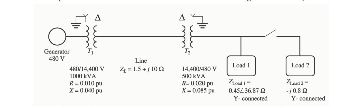
(a) Sketch the per-phase equivalent circuit of this power system. (b) With the switch opened, find the real power P, reactive power Q, and apparent power S supplied by the generator. What is the power factor of the generator? (c) With the switch closed, find the real power P, reactive power Q, and apparent power S supplied by the generator. What is the power factor of the generator? (d) What are the transmission losses (transformer plus transmission line losses) in this system with the switch open? With the switch closed? What is the effect of adding Load 2 to the system?
Solution
We select system base quantities in Region 1: Sbase1=1000 kVAVLL,base1=480 V
The base voltages and impedances for the three regions are:
- Region 1: Sbase1=1000 kVA, VLL,base1=480 V, Vϕ,base1=277 V Zbase1=1000 kVA3(277 V)2=0.238Ω
- Region 2: Sbase2=1000 kVA, VLL,base2=14,400 V, Vϕ,base2=8314 V Zbase2=1000 kVA3(8314 V)2=207.4Ω
- Region 3: Sbase3=1000 kVA, VLL,base3=480 V, Vϕ,base3=277 V Zbase3=1000 kVA3(277 V)2=0.238Ω
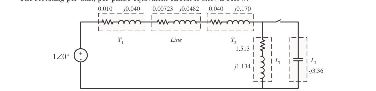
(a) Per-Phase Per-Unit Equivalent Circuit
Transformer T1 impedance (1000 kVA base): R1,pu=0.010 puX1,pu=0.040 pu
Transformer T2 impedance (500 kVA base, converted to 1000 kVA base): R2,pu=0.020×(500 kVA1000 kVA)=0.040 pu X2,pu=0.085×(500 kVA1000 kVA)=0.170 pu
Transmission line impedance (Zline=1.5+j10.0Ω in Region 2): Zline,pu=207.4Ω1.5+j10.0Ω=0.00723+j0.0482 pu
Load 1 impedance (Zload1=0.45∠36.87∘Ω in Region 3): Zload1,pu=0.238Ω0.45∠36.87∘Ω=1.513+j1.134 pu
Load 2 impedance (Zload2=−j0.8Ω in Region 3): Zload2,pu=0.238Ω−j0.8Ω=−j3.36 pu
The resulting per-unit per-phase equivalent circuit is:
(b) Switch Open (Load 1 Only)
Total equivalent impedance: ZEQ=(0.010+j0.040)+(0.00723+j0.0482)+(0.040+j0.170)+(1.513+j1.134) ZEQ=1.5702+j1.3922 pu=2.099∠41.6∘ pu
Generator current: I=2.099∠41.6∘1.0∠0∘ pu=0.4765∠−41.6∘ pu
Load voltage: VLoad,pu=IZload1=(0.4765∠−41.6∘)(1.513+j1.134)=0.901∠−4.7∘ pu VLoad=0.901(480 V)=432 V
Power to load: PLoad,pu=I2Rload1=(0.4765)2(1.513)=0.344 pu⟹PLoad=344 kW
Power supplied by generator: PG=VIcosθ=(1.0)(0.4765)cos41.6∘=0.356 pu⟹PG=356 kW QG=VIsinθ=(1.0)(0.4765)sin41.6∘=0.316 pu⟹QG=316 kvar SG=VI=(1.0)(0.4765)=0.4765 pu⟹SG=476.5 kVA PFG=cos41.6∘=0.748 lagging
(c) Switch Closed (Both Loads Connected)
Parallel combination of Load 1 and Load 2: ZL,tot=1.513+j(1.134−3.36)(1.513+j1.134)(−j3.36)=2.358+j0.109 pu
Total system impedance: ZEQ=(0.010+j0.040)+(0.00723+j0.0482)+(0.040+j0.170)+(2.358+j0.109) ZEQ=2.415+j0.367 pu=2.443∠8.65∘ pu
Generator current: I=2.443∠8.65∘1.0∠0∘ pu=0.409∠−8.65∘ pu
Load voltage: VLoad,pu=(0.409∠−8.65∘)(2.358+j0.109)=0.966∠−6.0∘ pu VLoad=0.966(480 V)=464 V
Power to loads: PLoad,pu=(0.409)2(2.358)=0.394 pu⟹PLoad=394 kW
Power supplied by generator: PG=(1.0)(0.409)cos6.0∘=0.407 pu⟹PG=407 kW QG=(1.0)(0.409)sin6.0∘=0.0428 pu⟹QG=42.8 kvar SG=0.409 pu⟹SG=409 kVA PFG=cos6.0∘=0.995 lagging
(d) Transmission Loss Comparison
Transmission losses with switch open: Ploss,pu=I2Rline=(0.4765)2(0.00723)=0.00164 pu⟹Ploss=1.64 kW
Transmission losses with switch closed: Ploss,pu=(0.409)2(0.00723)=0.00121 pu⟹Ploss=1.21 kW
Adding the capacitive load (Load 2) improved the system power factor from 0.748 lagging to 0.995 lagging. This increased the load voltage from 432 V to 464 V, increased total real power supplied to the loads from 344 kW to 394 kW, reduced generator apparent power from 476.5 kVA to 409 kVA, and reduced transmission losses from 1.64 kW down to 1.21 kW. This demonstrates the classic benefits of power factor correction in electric power transmission.